Latest trends in automobile industry, Which are the top family cars for your weekend trip?
This week, I will analyze Car Fuel Economy dataset from TidyTuesday.
What is TidyTuesday?
TidyTuesday is a weekly social data project in R organized by the R for Data Science community.
It is a great way of improving your Data wrangling and visualization techniques, sharing and learning from others.
You can find more information on their github.
Fuel economy data are the result of the work done by the US Environmental Protection Agency. Full data dictionary can be found at fueleconomy.gov.
The data contains 83 parameters of more than 40.000 Vehicles. That’s a lot of information!
Going for your next family camping adventure? First, check your car model.
Better Fuel economy and recent developments on longer running electric car batteries are great. But one thing which does not change in families’ lives is the need for space.
If you don’t want crying kids running around because of a missing teddy bear which did not fit in the baggage. Check, which brands will serve you best.
Especially, if you have a daughter who likes to travel with a lot of toys.
Let’s figure out a solution for peaceful weekend trip.
Which brand produce most family friendly cars? In terms of baggage volume.
library(tidyverse) # ggplot2, dplyr, tidyr, readr,
                   # purrr, tibble, stringr, forcats
big_epa_cars <- read_csv("https://raw.githubusercontent.com/rfordatascience/tidytuesday/master/data/2019/2019-10-15/big_epa_cars.csv")
dim(big_epa_cars)
## [1] 41804 83I will subset my data for easier computation.
Let’s keep the following columns:
- year - model year
- make - manufacturer (division)
- model - model name (carline)
- VClass - EPA vehicle size class
- hlv - hatchback luggage volume (cubic feet)
- hpv - hatchback passenger volume (cubic feet)
- displ - engine displacement in liters
- lv4 - 4 door luggage volume (cubic feet)
- pv4 - 4-door passenger volume
big_sub <- big_epa_cars %>%
  select(fuelType, year, make, model, VClass, hlv, hpv,lv4,pv4,displ)
I will start exploring the data. For the moment, first I will focus on Midsize cars (VClass).
I will filter for the main pool of Midsize cars with 4 door and luggage volume of bigger than 6 and passenger volume larger than 75.
posn.j <- position_jitter(width=0.2)
big_sw <- big_sub %>%
  filter(VClass == "Midsize Cars" & pv4 > 75 & lv4 > 6)

big_sw %>%
  ggplot(aes(x=pv4, y=lv4)) +
  geom_point(shape=21,
             alpha=0.4,size =3,
             position = posn.j) +
  theme(plot.caption=element_text(size=11),
        text = element_text(size=18),
        plot.title = element_text(size=32),
        legend.position = "none") +
  geom_smooth(method = "lm", color ="red") +
  coord_fixed() +
    labs(x = "Passenger Vol (Cubic feet)",
         y = "Luggage Vol (Cubic feet)",
         title =
    "Luggage space negatively \ncorrelates with passenger space")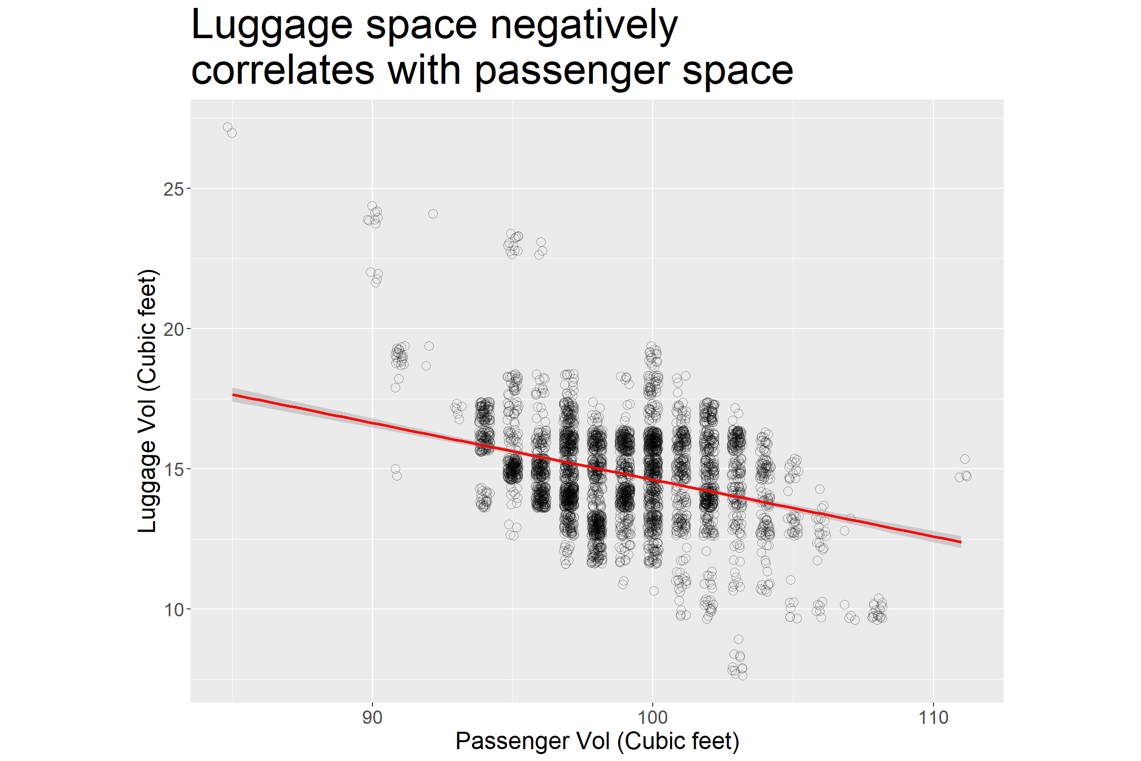
This is not unexpected. But good to see.
Insight 1: Negative correlation suggests that producers sacrifice passenger space to produce bigger room for the luggage or vice versa.
First, I will look at the luggage volume in Mid sized cars and I will order them according to highest average.
pp <- big_sw %>%
  mutate(make = fct_reorder(make, lv4)) %>%
  ggplot(aes(x=make, y=lv4, col=make)) +
  geom_boxplot(varwidth=TRUE) +
  theme(plot.caption=element_text(size=11),
        text = element_text(size=18),
        plot.title = element_text(size=32),
        legend.position = "none") +
  coord_flip() +
  labs(x = element_blank(),
       y = "Luggage size (cubic feet)",
       title = "Average luggage volumes in Midsized cars")
  pp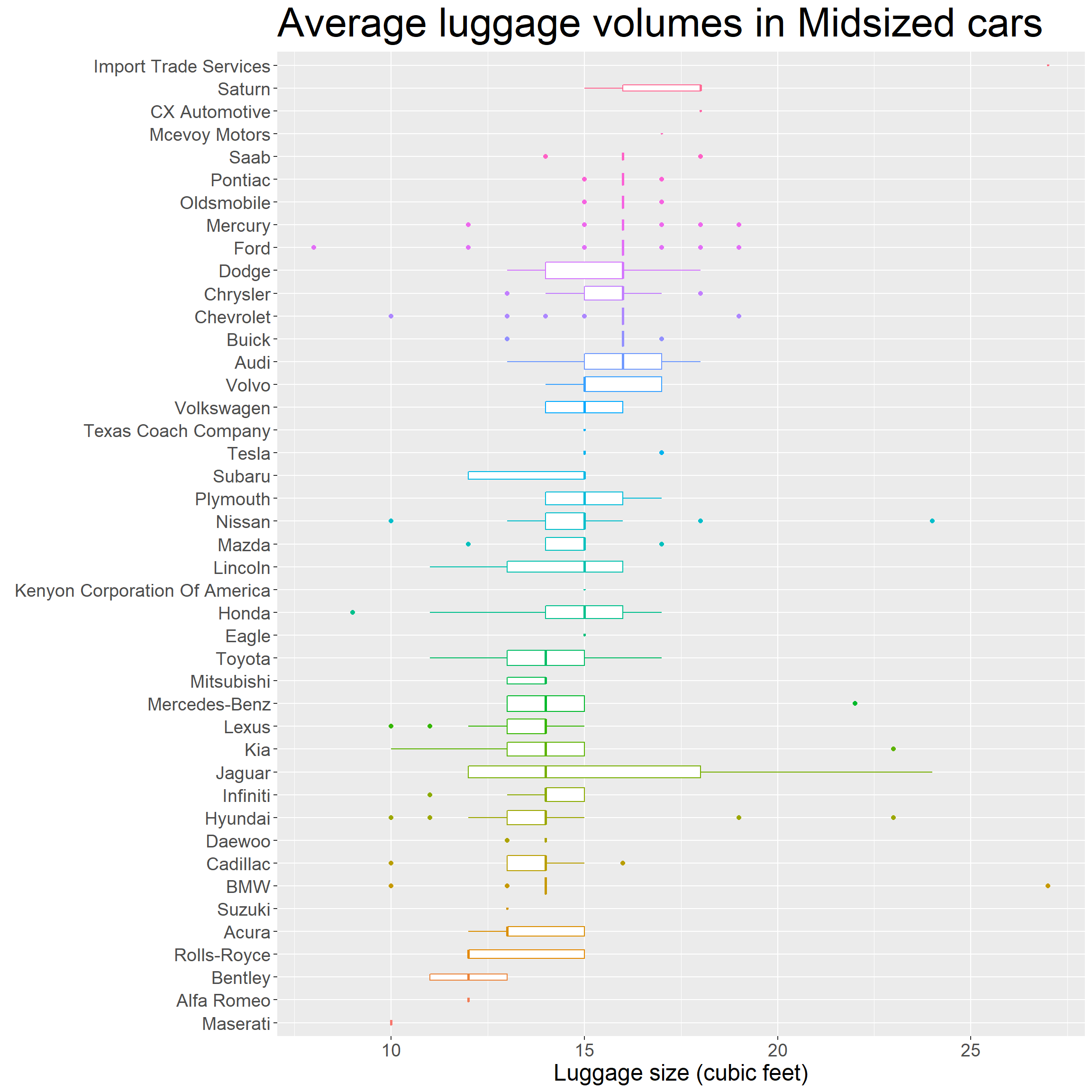
If you follow the mean lines from bottom to top, you will see that cars cluster into three groups according to their mean of luggage sizes. But differences are not huge.
Insight 2: Cars cluster into three groups according to their mean luggage size.
Let’s focus. I am looking for the car with the biggest luggage space. Let’s see what other VClass types are in our dataset that we can include our exploration.
There are 34 types of vehicle classes (Vlass) in our dataset. I will subset all the relevant ones, leaving some specialty vehicles and vans aside.
You can have a look at other VClass types with this code here.
big_epa_cars %>% group_by(VClass) %>% count() %>% arrange(desc(n))
I will also remove minor brands with less than 10 models in total.
big_filtered <- big_sub %>%
  filter(VClass %in% c("Large Cars", "Compact Cars", "Midsize Cars",
                       "Midsize Station Wagons", "Midsize-Large Station Wagons",
                       "Minivan - 2WD", "Minivan - 4WD")) %>%
  group_by(make) %>%
  mutate(n=n()) %>%
  filter(n > 10) %>%
  ungroup()

dim(big_filtered)
## [1] 14710 11To be on the safe side for the family trip, I will choose cars not older than 5 years.
# Cars ordered with luggage volume, but not older than 5 years
# and lv4 bigger than 5

q <- big_filtered %>%
  filter(year > 2016, lv4 > 5) %>%
  mutate(make = fct_reorder(make, lv4)) %>%
  ggplot(aes(x=make, y=lv4, col=make)) +
  geom_boxplot(varwidth=TRUE) +
  theme(text = element_text(size=15),
        legend.position = "none") +
  coord_flip()
q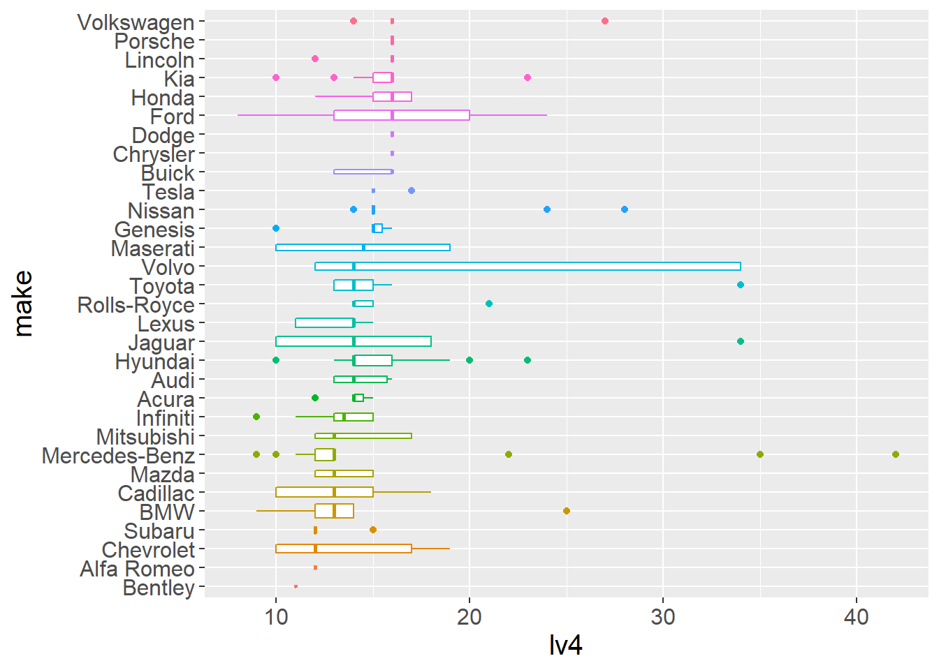
There are not big differences between average luggage size of different brands. Although, you will probably get more space if you choose a Volkswagen or Ford rather than a BMW or Chevrolet.
The real XL luggage volume cars are plenty and seem to be more outlier models. To find our dream car let’s focus on those outliers.
I will create a new data frame boot_space containing the top 50 cars according to the luggage volume.
boot_space <- big_filtered %>%
  filter(year > 2016) %>%
  arrange(desc(lv4)) %>%
  top_n(50, lv4)

# Top family cars - geom_point()
bs <- boot_space %>%
  mutate(model = fct_reorder(model, lv4)) %>%
  mutate(make = fct_reorder(make, lv4)) %>%
  ggplot(aes(x=make,y= model, size=lv4, col=VClass)) +
  geom_point() +
  theme(plot.caption=element_text(size=12),
        axis.text.x=element_text(angle=45, hjust=1),
        text = element_text(size=18),
        plot.title = element_text(size=32)) +
labs(caption= "Data: https://fueleconomy.gov",
     size="Luggage Vol\n(Cubic feet)",
     x = element_blank(),
     y = element_blank(),
     title = "Which are the best family cars?") +
  guides(size = guide_legend(order = 1),
         shape = guide_legend(order = 2)) +
  scale_size(range=c(2, 9))
bs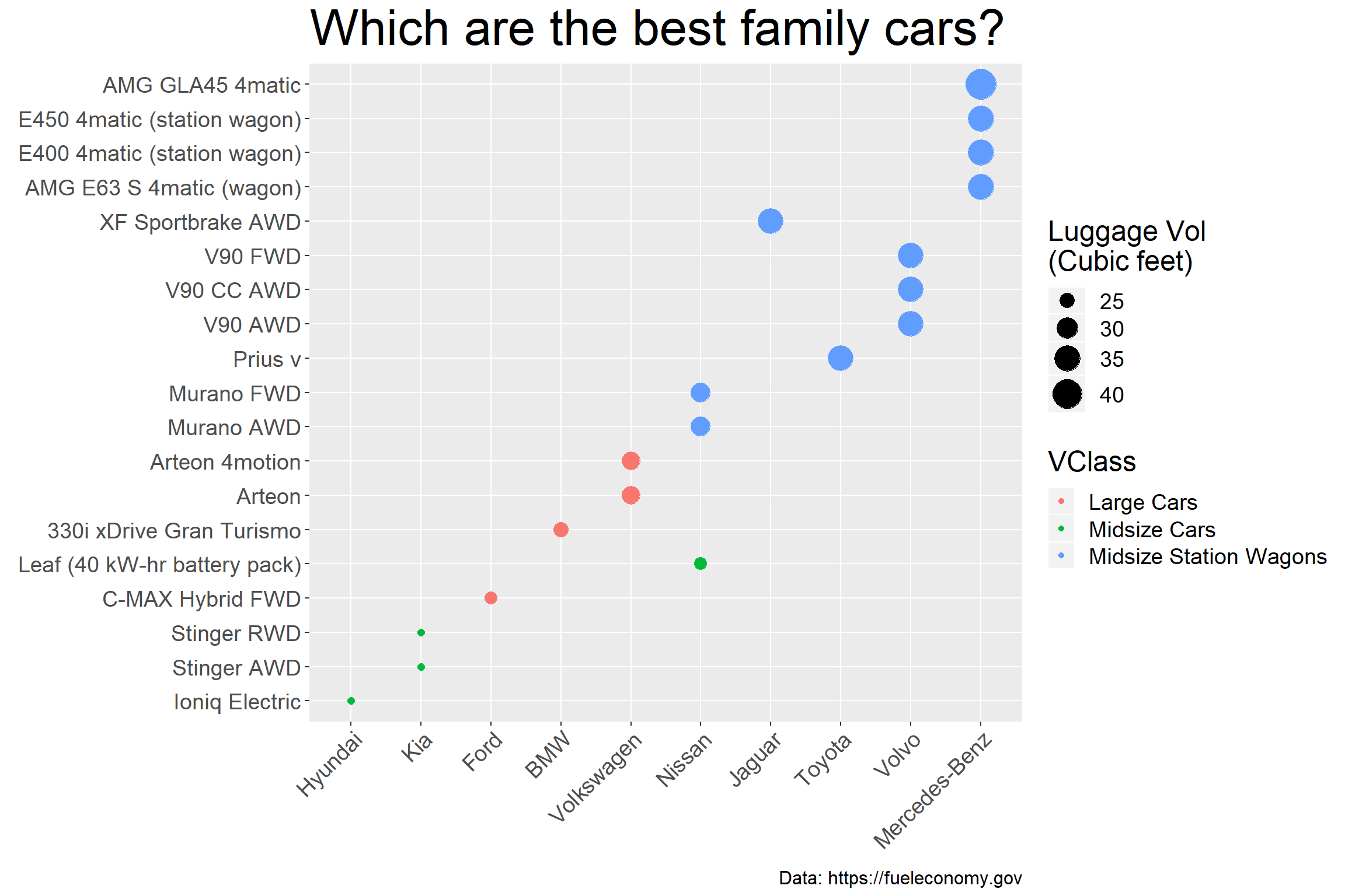
Mercedes AMG GLA45 is the winner with 42 cubic feet space!
Here is another presentation, for easier comparision.
# Top family cars - geom_Col()
bs_col <- boot_space %>%
    mutate(model = fct_reorder(model, lv4)) %>%
    mutate(make = fct_reorder(make, lv4)) %>%
    ggplot(aes(x=model, y=lv4, fill=make)) +
    geom_col(position="dodge")+coord_flip() +
    theme(plot.caption=element_text(size=11),
          text = element_text(size=18),
          plot.title = element_text(size=32)) +
labs(caption= "Data source: https://fueleconomy.gov",
     size="Luggage Vol\n(Cubic feet)",
     x = element_blank(),
     y = "Luggage Vol (Cubic feet)",
     title = "Which are the best family cars?") +
    scale_size(range=c(2, 9))

bs_col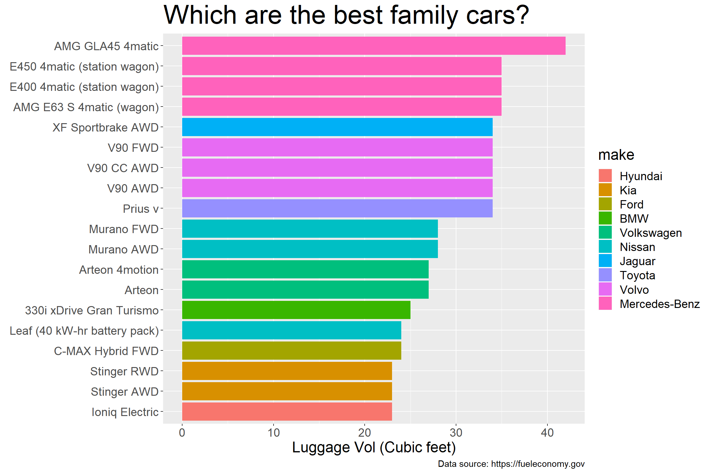
We found our answer and our camping gear is ready. Let’s tackle some other questions. We hear a lot about them but how does the future looks like for Electric cars?
How do Electric cars evolving in the last years compared to non electric cars?
There are many of different types of engines capable of using one or two different fuel sources. Let’s look at how their numbers compare during the last years.
# Using Varwidth: Ordered
pp  <- big_epa_cars %>%
  mutate(fuelType=fct_reorder(fuelType, year)) %>%
  ggplot(aes(x=fuelType, y =year, fill=fuelType)) +
  geom_boxplot(varwidth=TRUE) +
  coord_flip() +
  theme(legend.position = "none",
        text = element_text(size=18),
        plot.title = element_text(size=32),
        axis.text.x = element_text(angle = 45, hjust = 1)) +
  labs(x = "Fuel Type",
       y = "Year",
       title =
         "How does prominence of Fuel Types \nchange with the year?")

pp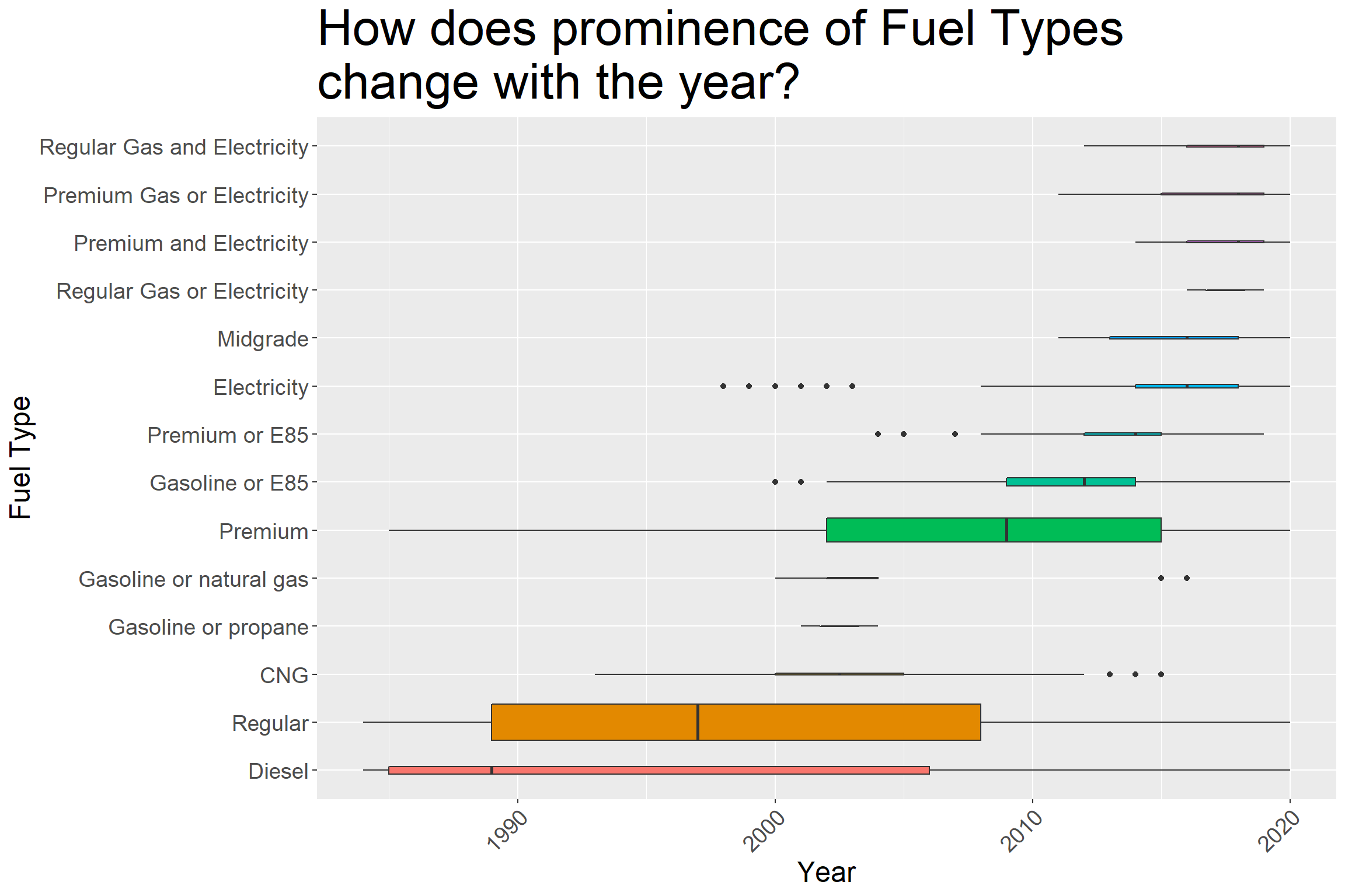
Group Electric vs Non Electric cars
I will group cars whehter or not they can use electricity.
# Grouped: Electric vs no electric:
big_epa_cars$fuelType <- ifelse(big_epa_cars$fuelType %in%
               c("Regular Gas and Electricity",
                "Premium Gas or Electricity",
                 "Premium and Electricity",
                "Regular Gas or Electricity",
                "Electricity"), "Electric", "Non-Electric")

pp  <- big_epa_cars %>%
  mutate(fuelType=fct_reorder(fuelType, year)) %>%
  ggplot(aes(x=fuelType, y =year, fill=fuelType)) +
  geom_boxplot(varwidth=TRUE) +
  coord_flip() +
  theme(text = element_text(size=18),
        plot.title = element_text(size=32), legend.position = "none")+
  theme(text = element_text(size=15)) +
  labs(x = "Fuel Type",
       y = "Year",
       title = "How does prominence of Fuel Types \nchange with the year?")

pp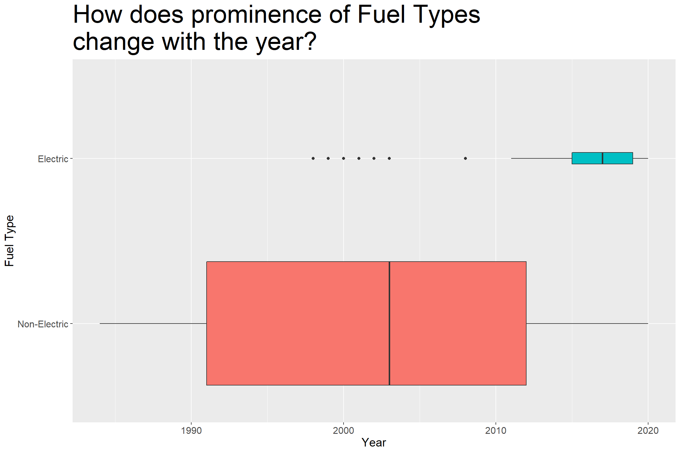
In the last couple of years, number of electric car models are increasing but they are still a minority.
big3 <- big_epa_cars %>%
  group_by(year, fuelType) %>%
  mutate(n = n())

big3 %>%
    ggplot(aes(x=n, y =year, col=fuelType)) +
    geom_point(size=4) +
    theme(legend.position = c(0.9,0.9),
          legend.title= element_blank(),
          legend.background = element_blank(),
          plot.title = element_text(size=32),
          text = element_text(size=15)) +
  coord_flip() +
    labs(x = "Number of Car models",
         y = "Year",
         title = "How does the Numbers of Electric vs Non Electric cars \nchange by year?")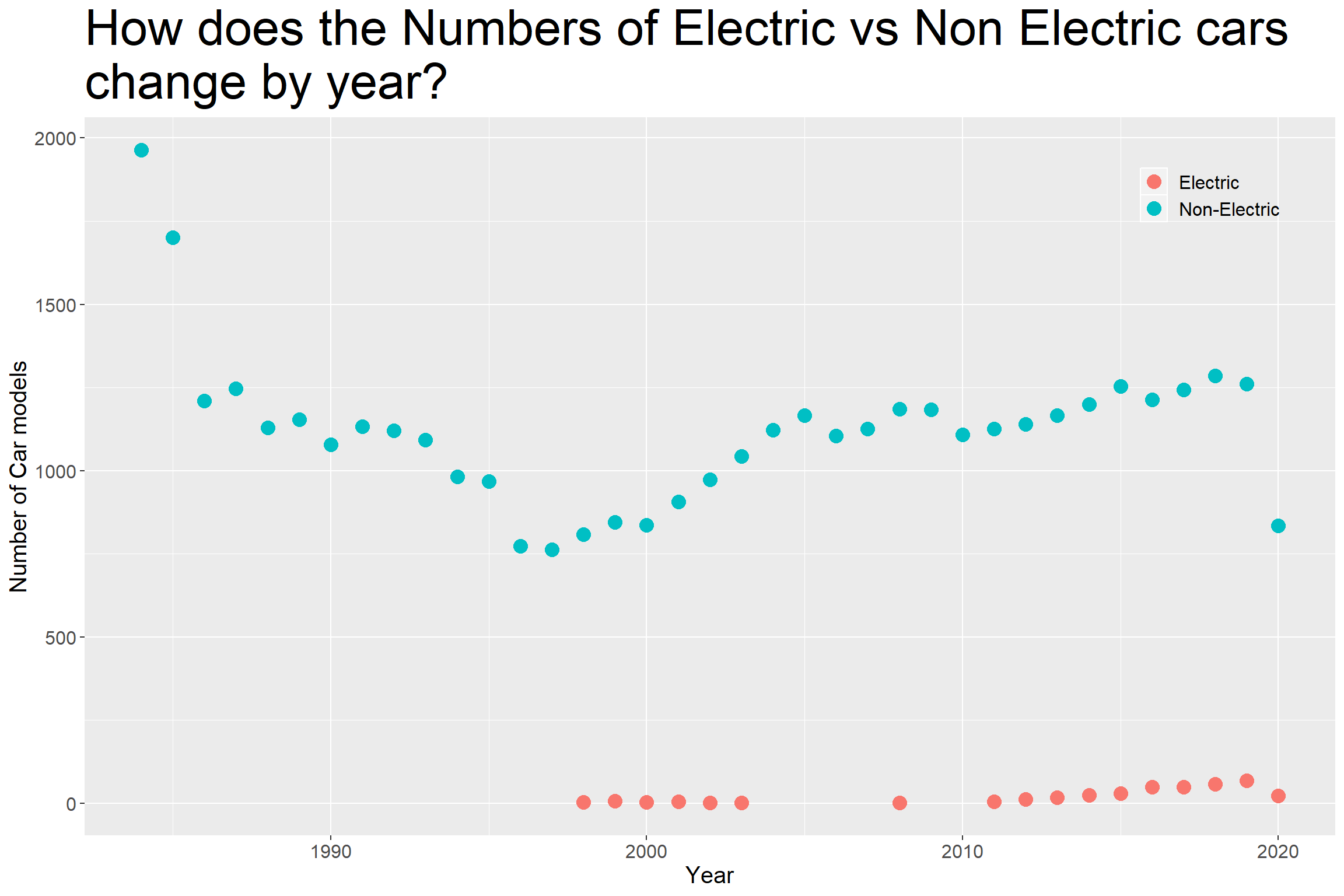
Both Electric and Non Electric car models follows a similar increase in the last 10 years
Increases in Electric car models in the last years might be a reflection of a general increase in total number of model types
Conclusions / Future thoughts
This was a huge dataset. You can answer many other questions such as mileage of different car models, carbon dioxide emissions, fuel savings.
I have selected some car models which might be a good option if luggage space is a priority for you!
To see other examples of how people used this dataset follow the Twitter hashtag #TidyTuesday.
Please share if you have other ideas in the comments below!
Until next time!
Serdar
Serdar Korur
Data Scientist and PhD in Molecular Biology
Serdar is a Data Scientist and PhD in Cell Biology