Data Preparation: Web Scraping html tables with rvest
Accessing different data sources
Sometimes, the data you need is available on the web. Accessing those will ease your life as a data scientist.
I want to perform an exploratory data analysis on 2018/19 Season of England Premier league.
- Are there changes in team performances during the season timeline?
- Does some teams cluster?
- Which is the earliest week we can predict team’s final positions?
I need the standings table for each week of the season and integrate them in a way that will allow me to plot the graphs that I want.
We will scrap those tables from https://www.weltfussball.de/.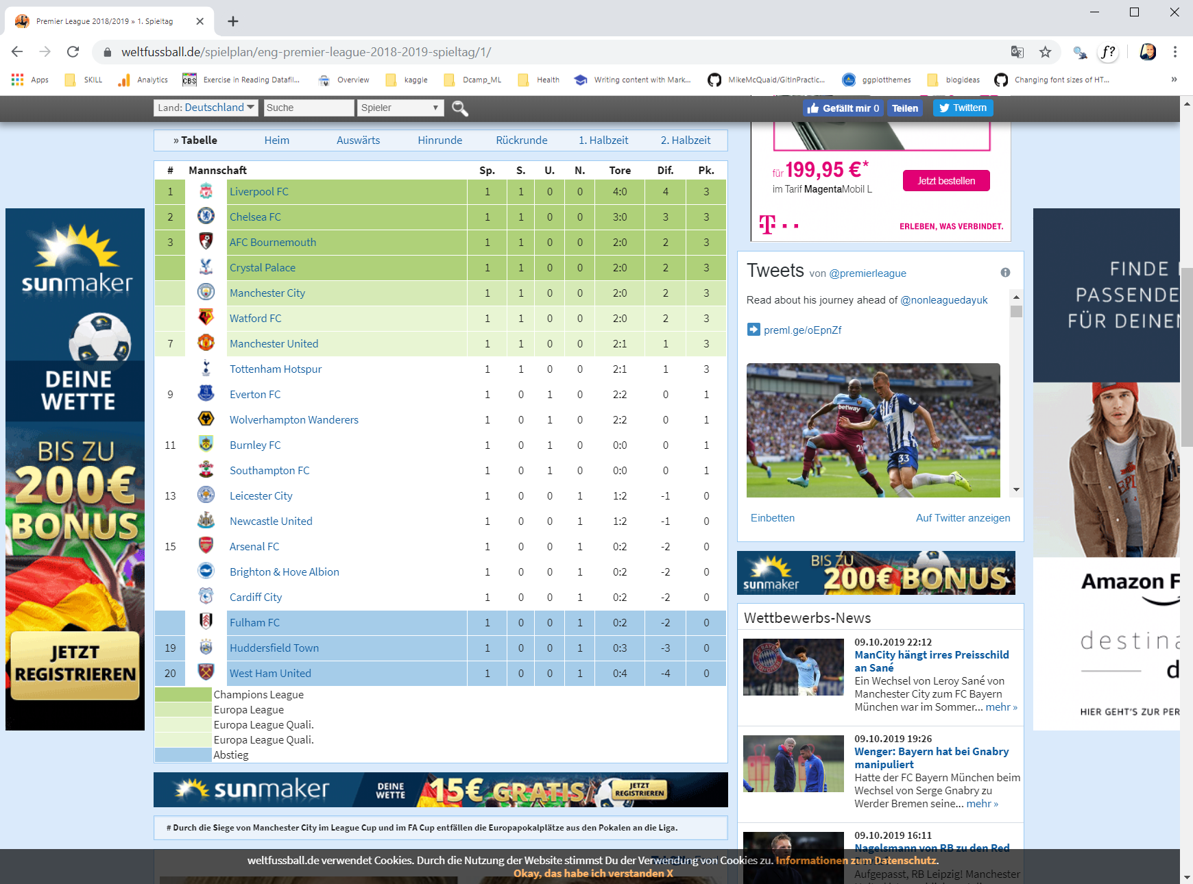
For example standings table for the Week 1 is at the url:
https://www.weltfussball.de/spielplan/eng-premier-league-2018-2019-spieltag/1
For the consequent weeks only the number at the end changes e.g.
../spielplan/eng-premier-league-2018-2019-spieltag/2 ←
../spielplan/eng-premier-league-2018-2019-spieltag/3 ←
# Pull the necessary packages

library(rvest)     # xml2
library(tidyverse) # ggplot2, dplyr, tidyr, readr,
                   # purrr, tibble, stringr, forcats
library(gganimate)
library(RColorBrewer)
library(kableExtra)
# Define the remote url
baseUrl <- "https://www.weltfussball.de/"
path <- "spielplan/eng-premier-league-2018-2019-spieltag/"
fileName <- 1
url <- paste0(baseUrl, path, fileName)
url## [1] "https://www.weltfussball.de/spielplan/eng-premier-league-2018-2019-spieltag/1"We start by downloading and parsing the file with read_html() function from the rvest package.
tables <- read_html(url)To extract the html table individually you can use XPath syntax which defines parts on XML documents.
To get the XPath for standings table open the url on google chrome,
- hover the mouse over the table > right click > inspect
# This will open inspector - Move your mouse a few lines up or down to find the line where whole table is highlighted
- Right click > Copy > Copy full XPath
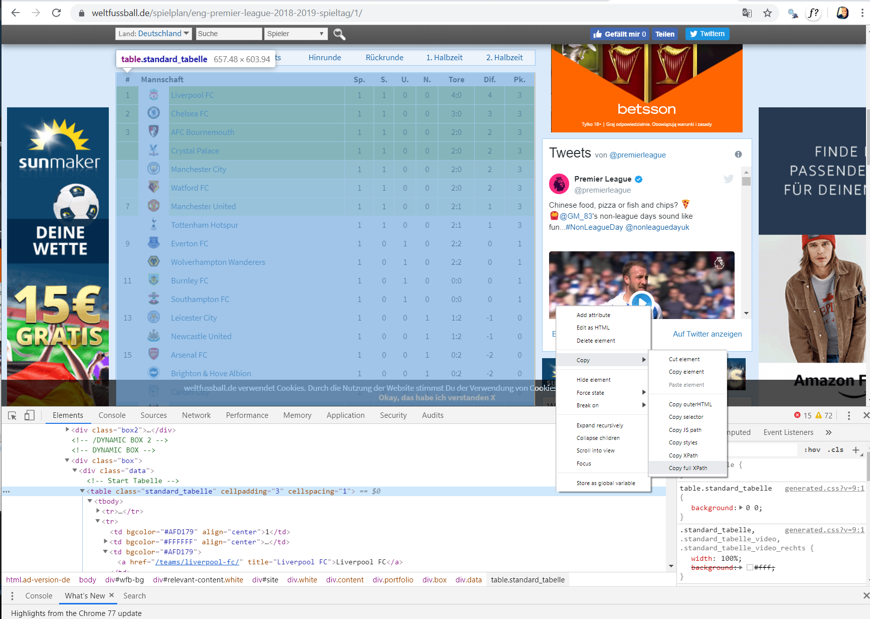
We can feed that XPath we copied to html_nodes() function and extract the node which contains the table.
xpath = "/html/body/div[3]/div[2]/div[4]/div[2]/div[1]/div/div[7]/div/table[1]"
nodes <- html_nodes(tables, xpath = xpath)
At the end, html_table() function will extract us the individual table.
html_table(nodes)## [[1]]
## # Mannschaft Mannschaft Sp. S. U. N. Tore Dif. Pk.
## 1 1 NA Liverpool FC 1 1 0 0 4:0 4 3
## 2 2 NA Chelsea FC 1 1 0 0 3:0 3 3
## 3 3 NA AFC Bournemouth 1 1 0 0 2:0 2 3
## 4 NA NA Crystal Palace 1 1 0 0 2:0 2 3
## 5 NA NA Manchester City 1 1 0 0 2:0 2 3
## 6 NA NA Watford FC 1 1 0 0 2:0 2 3
## 7 7 NA Manchester United 1 1 0 0 2:1 1 3
## 8 NA NA Tottenham Hotspur 1 1 0 0 2:1 1 3
## 9 9 NA Everton FC 1 0 1 0 2:2 0 1
## 10 NA NA Wolverhampton Wanderers 1 0 1 0 2:2 0 1
## 11 11 NA Burnley FC 1 0 1 0 0:0 0 1
## 12 NA NA Southampton FC 1 0 1 0 0:0 0 1
## 13 13 NA Leicester City 1 0 0 1 1:2 -1 0
## 14 NA NA Newcastle United 1 0 0 1 1:2 -1 0
## 15 15 NA Arsenal FC 1 0 0 1 0:2 -2 0
## 16 NA NA Brighton & Hove Albion 1 0 0 1 0:2 -2 0
## 17 NA NA Cardiff City 1 0 0 1 0:2 -2 0
## 18 NA NA Fulham FC 1 0 0 1 0:2 -2 0
## 19 19 NA Huddersfield Town 1 0 0 1 0:3 -3 0
## 20 20 NA West Ham United 1 0 0 1 0:4 -4 0Wonderful, we scraped the standings table for the first week, but we want tables for each 38 week of the season.
You can make this easily by packing what we have done so far in a for loop.
As only the last number in our url link changes, we can code different url addresses as in url[[i]] <- paste0(baseUrl, path, i)
# Create emtpy lists
url <- list()
pages <- list()
nodes <- list()
final <- list()
start <- Sys.time()
# For loop.
# It will connect one by one to 38 different url links predefined
# by the line starting with url[[i]]
# Collect the information with read_html(), html_nodes() and html_table()
# Finally each table will be converted to a data frame
for(i in 1:38){
url[[i]] <- paste0(baseUrl, path, i)
pages[[i]] <- read_html(url[[i]])
nodes[[i]] <- html_nodes(pages[[i]], xpath = xpath)
final[[i]] <- data.frame(html_table(nodes[[i]]))
}

# By coding start and end times of the whole process
# I can keep an eye on how fast my code is.
end <- Sys.time()
end-start
## Time difference of 22.62705 secsFor example, final[[19]] will give me standings of mid season:
final[[19]]## X. Mannschaft Mannschaft.1 Sp. S. U. N. Tore Dif. Pk.
## 1 1 NA Liverpool FC 19 16 3 0 43:7 36 51
## 2 2 NA Tottenham Hotspur 19 15 0 4 42:18 24 45
## 3 3 NA Manchester City 19 14 2 3 51:15 36 44
## 4 4 NA Chelsea FC 19 12 4 3 37:16 21 40
## 5 5 NA Arsenal FC 19 11 5 3 41:25 16 38
## 6 6 NA Manchester United 19 9 5 5 37:31 6 32
## 7 7 NA Leicester City 19 8 4 7 24:22 2 28
## 8 8 NA Everton FC 19 7 6 6 31:29 2 27
## 9 9 NA West Ham United 19 8 3 8 27:28 -1 27
## 10 10 NA Watford FC 19 8 3 8 26:27 -1 27
## 11 11 NA Wolverhampton Wanderers 19 7 5 7 20:22 -2 26
## 12 12 NA AFC Bournemouth 19 8 2 9 27:33 -6 26
## 13 13 NA Brighton & Hove Albion 19 6 4 9 21:27 -6 22
## 14 14 NA Crystal Palace 19 5 4 10 17:25 -8 19
## 15 15 NA Newcastle United 19 4 5 10 14:26 -12 17
## 16 16 NA Southampton FC 19 3 6 10 20:35 -15 15
## 17 17 NA Cardiff City 19 4 3 12 18:38 -20 15
## 18 18 NA Burnley FC 19 3 3 13 17:41 -24 12
## 19 19 NA Fulham FC 19 2 5 12 17:43 -26 11
## 20 20 NA Huddersfield Town 19 2 4 13 12:34 -22 10Don’t mind the NAs in the second column, we will remove them soon. Now, we have all 38 table in our list final, we can combine them to a new data frame which will contain standings of the whole season.
To be able to plot e.g. timeline, let’s keep the tidy data principles:
- Each observation has its own row.
- Each variable has its own column.
Since we have same column names in each table, we can use rbind function to add rows of each table to the bottom of the first one. How to do that? We can’t use lapply() function here. It will not combine elements in a list. We can use do.call() function to perform the rbind() operation and combine all data frames we have*.
uk18 <-  do.call("rbind", final)
dim(uk18)
## [1] 760 10head(uk18)## X. Mannschaft Mannschaft.1 Sp. S. U. N. Tore Dif. Pk.
## 1 1 NA Liverpool FC 1 1 0 0 4:0 4 3
## 2 2 NA Chelsea FC 1 1 0 0 3:0 3 3
## 3 3 NA AFC Bournemouth 1 1 0 0 2:0 2 3
## 4 NA NA Crystal Palace 1 1 0 0 2:0 2 3
## 5 NA NA Manchester City 1 1 0 0 2:0 2 3
## 6 NA NA Watford FC 1 1 0 0 2:0 2 3Column names/shorcuts were in German, let’s replace them with the English words.
# Correct final table
uk18 <- uk18  %>% select(3:10)
new_names <- c("team", "week", "won", "drawn", "lost", "goals",
               "difference", "points")
colnames(uk18) <- new_names
Goals variable is contains two different data separated with “:”. E.g. (4:0). Those represent goals scored:goals scored against. Let’s split goals column into two by separate() function from tidyr.
uk18 <- uk18 %>% separate(goals, c("scored", "against"), sep="\\:")
head(uk18)
## team week won drawn lost scored against difference points
## 1 Liverpool FC 1 1 0 0 4 0 4 3
## 2 Chelsea FC 1 1 0 0 3 0 3 3
## 3 AFC Bournemouth 1 1 0 0 2 0 2 3
## 4 Crystal Palace 1 1 0 0 2 0 2 3
## 5 Manchester City 1 1 0 0 2 0 2 3
## 6 Watford FC 1 1 0 0 2 0 2 3I want to order my legend with the same order of teams final positions. Let’s filter for the last week of the season and arrange them in descending order. I will assign this list to the factor levels of the team variable.
# Extract team names in the order as the season end
uk18_filt <- uk18 %>%
  filter(week == 38) %>%
  arrange(desc(points))
knitr::kable(uk18_filt)| team | week | won | drawn | lost | scored | against | difference | points |
|---|---|---|---|---|---|---|---|---|
| Manchester City | 38 | 32 | 2 | 4 | 95 | 23 | 72 | 98 |
| Liverpool FC | 38 | 30 | 7 | 1 | 89 | 22 | 67 | 97 |
| Chelsea FC | 38 | 21 | 9 | 8 | 63 | 39 | 24 | 72 |
| Tottenham Hotspur | 38 | 23 | 2 | 13 | 67 | 39 | 28 | 71 |
| Arsenal FC | 38 | 21 | 7 | 10 | 73 | 51 | 22 | 70 |
| Manchester United | 38 | 19 | 9 | 10 | 65 | 54 | 11 | 66 |
| Wolverhampton Wanderers | 38 | 16 | 9 | 13 | 47 | 46 | 1 | 57 |
| Everton FC | 38 | 15 | 9 | 14 | 54 | 46 | 8 | 54 |
| Leicester City | 38 | 15 | 7 | 16 | 51 | 48 | 3 | 52 |
| West Ham United | 38 | 15 | 7 | 16 | 52 | 55 | -3 | 52 |
| Watford FC | 38 | 14 | 8 | 16 | 52 | 59 | -7 | 50 |
| Crystal Palace | 38 | 14 | 7 | 17 | 51 | 53 | -2 | 49 |
| Newcastle United | 38 | 12 | 9 | 17 | 42 | 48 | -6 | 45 |
| AFC Bournemouth | 38 | 13 | 6 | 19 | 56 | 70 | -14 | 45 |
| Burnley FC | 38 | 11 | 7 | 20 | 45 | 68 | -23 | 40 |
| Southampton FC | 38 | 9 | 12 | 17 | 45 | 65 | -20 | 39 |
| Brighton & Hove Albion | 38 | 9 | 9 | 20 | 35 | 60 | -25 | 36 |
| Cardiff City | 38 | 10 | 4 | 24 | 34 | 69 | -35 | 34 |
| Fulham FC | 38 | 7 | 5 | 26 | 34 | 81 | -47 | 26 |
| Huddersfield Town | 38 | 3 | 7 | 28 | 22 | 76 | -54 | 16 |
finallevels <- as.character(uk18_filt$team)
uk18$team <- factor(uk18$team, levels = finallevels)
You can also create a color palette which fits to your needs.
# We need a color palette with 20 colors
colorCount <- length(unique(uk18$team))
# colorRampPalette creatas a getPalette() function
# This can modify an existing palette to include as many colors we want
getPalette <- colorRampPalette(brewer.pal(9, "Set1"))
getPalette(colorCount)
## [1] "#E41A1C" "#9B445D" "#526E9F" "#3C8A9B" "#469F6C" "#54A453" "#747B78"
## [8] "#94539E" "#BD6066" "#E97422" "#FF990A" "#FFCF20" "#FAF632" "#D4AE2D"
## [15] "#AF6729" "#BF6357" "#E17597" "#E884B9" "#C08EA9" "#999999"# Plot season timeline using the palette we just created
uk <- ggplot(uk18, aes(x=week, y=points, col=team)) +
geom_point(size=3) +
theme(text = element_text(size=15)) +
scale_color_manual(values = getPalette(colorCount))Let’s plot the regression lines
# Plot season timeline
uk <- ggplot(uk18, aes(x=week, y=points, col=team)) +
  geom_smooth(se=TRUE) +
  theme(text = element_text(size=15)) +
  scale_color_manual(values = getPalette(colorCount))

uk
## `geom_smooth()` using method = 'loess' and formula 'y ~ x'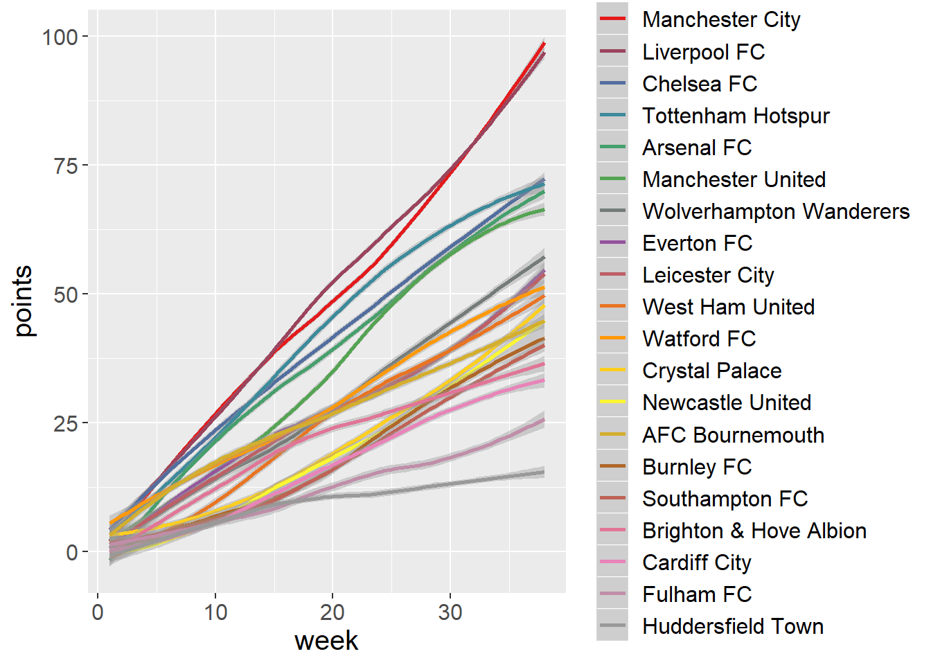
uk_facet <- ggplot(uk18, aes(x=week, y=points, col=team)) +
  geom_smooth(se=FALSE) +
  theme(text = element_text(size=10)) +
  scale_color_manual(values = getPalette(colorCount)) +
  facet_wrap(ncol = 4, team~.)

uk_facet
## `geom_smooth()` using method = 'loess' and formula 'y ~ x'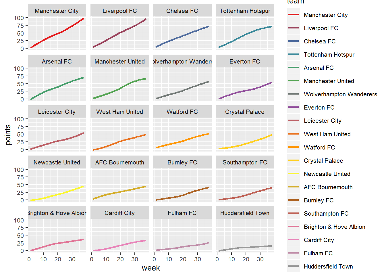 Some insights from the plots:
- I see three clusters here. Two teams (Man. City and Liverpool) competed head to head for the championship and next three teams (Chelsea, Tottenham and Arsenal) for the 3rd position.
- We can predict 4 out of 5 teams which will take first 5 place at the end of the season early as week 10.
- Manchester United showed peak performance mid season, Everton have improved performances while Tottenham slowed down (which costed them 3rd position) in the second part of the season.
I can plot points against goal differences in the same plot. Same clusters pop up here as well.
uk <- ggplot(uk18, aes(x=difference, y=points, col=team)) +
  geom_point(size=2) +
  scale_color_manual(values = getPalette(colorCount)) +
  theme(text = element_text(size=15))
uk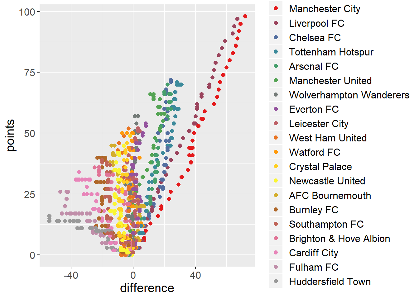
Let’s visualize this in a small animation. You can create an animated plot of the teams progress during the season. Gganimate does good job.`
# Add a shadow tail
# anim + shadow_wake(wake_length = 0.3, alpha = FALSE)

anim <- uk +
             transition_time(week) +
             labs(title = "week: {round(frame_time,0)}") +
             shadow_wake(wake_length = 0.1, alpha = 0.5)

fullanimation <- animate(anim, fps= 7, nframes=100,
                         height=500, width=800, res=0.8)

fullanimation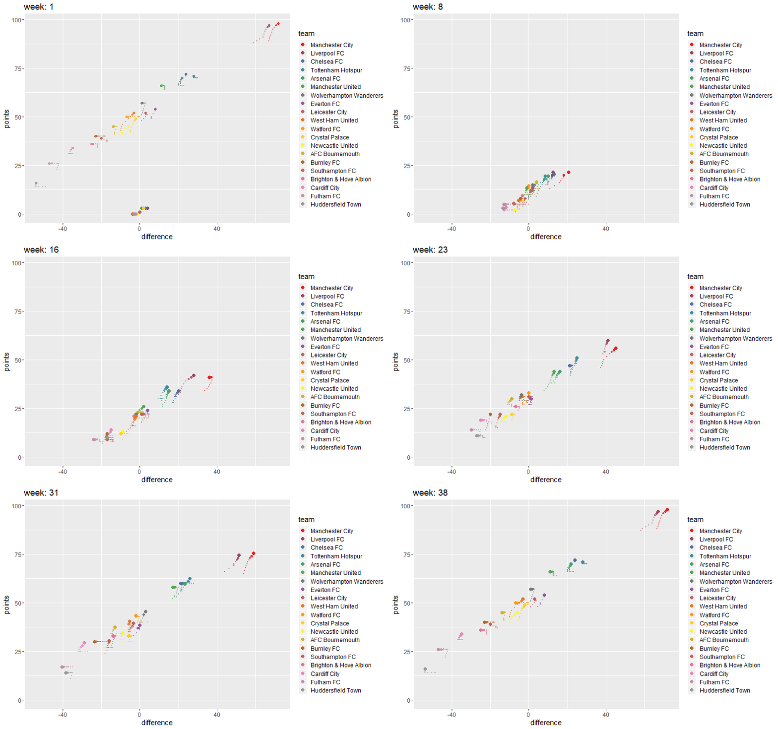
Conclusions / Future Thoughts
One of the most important steps to answer a research question is gathering and pre-processing data that fits best for the planned analysis.
Some of the questions we tackled were:
- How to find the XPath for an html table in a website?
- How to combine data frames from a list?
- How to split columns containing more than one variable?
The earliest time, we can predict top teams final positions was around 10th. We can collect data from previous years or compare other countries leagues to check if we can generalize this finding.
What else we can ask? For example, we can connect performance changes to new transfers. Or whether changing coaches benefited any team.
As we saw web is a great source for data. If you want to use it more effectively, learn about different data formats such as JSON or XML and interact with APIs, here is a great course from Datacamp.
Please share if you have other ideas in the comments below!
Until next time!
Serdar
PS: If you are looking for more blogs to learn R you might check also: