An intuitive real life example of a binomial distribution and how to simulate it in R: Learn it once, use it everyday
Learn. It is all about success and failure.
What are binomial distributions and why are they so useful?
When we repeat a set of events like 10 times coin flipping and each single event in a set has two possible outcomes (head or tails) think about Binomial distributions. Each single event here is known as a Bernoulli Trial.
Bi- in binomial distributions refers to the two outcomes usually described as Success or no Success. A “yes” or “no”.
Probability distributions in general are used to predict future events and often based on nasty looking mathematical formulas. But, there is also a beautiful thing here. For example the specific binomial distribution mathematical function can be used to predict the outcomes of any real life event which has two outcomes.
Let’s start with a simple example.
Why is this interesting?
For example, playing with the coins, the two possibilities are getting heads (success) or tails (no success). And let’s say you have a of e.g. 50 times coin flipping. We can repeat this set as many times as we like and record how many times we got heads (success) in each repetition.
And if plot the results we will have a probability distribution plot. And if you make enough repetitions you will approach a binomial probability distribution curve. We will do this in a minute. But, first generate data to draw our plot.
We can use R to generate the data. We will generate random data from repeating set of 50-times coin flipping 100000 times and record the number of successes in each repetition.
rbinom() function can generate a given number of repeated (here 100.000) sets (50 times of coin flipping) of experiments. It requires 3 arguments.
rbinom(
n = number of repetitions = 100.000,
size = sample size = 50,
p = the probability of success (chance of throwing heads is 0.5))
R code can be used to find the exact probabilities. Let’s compare the probabilities of getting more than 25, 35 or even 49 heads. You can combine rbinom with mean function to find the percentage of the events with a chosen outcome.
# Probability of getting 25 or more heads
mean(rbinom(100000, 50, .5) >= 25)
## [1] 0.55734# Probability of getting 35 or more heads
mean(rbinom(100000, 50, .5) >= 35)## [1] 0.00358# Probability of getting 49 or more heads
mean(rbinom(100000, 50, .5) >= 49)## [1] 0We found the probability of throwing 49 or more heads to be 0. But to be technically precise it is one in 375 trillion times (= \(1/((1/(2^{49}) + (1/2^{50})))\)).
Let’s visualize our simulation. The bars in red represents the sets which had 35 or more heads.
library(tidyverse) # ggplot2, dplyr, tidyr, readr,
                   # purrr, tibble, stringr, forcats
library(viridis)

heads <- rbinom(100000, 50, 0.5)
heads <- data.frame(heads)
heads <- heads %>% mutate(events = ifelse(heads > 35, "> 35", "< 35"))
heads %>%  ggplot(aes(x=heads, fill = events)) +
  geom_histogram(binwidth = 0.5) +
  scale_fill_manual(values = c("black", "red")) +
  theme_classic() +
  theme(text = element_text(size = 18),
        legend.position = c(0.85, 0.85)) +
  labs(x = "Number of heads in 50 coin flips")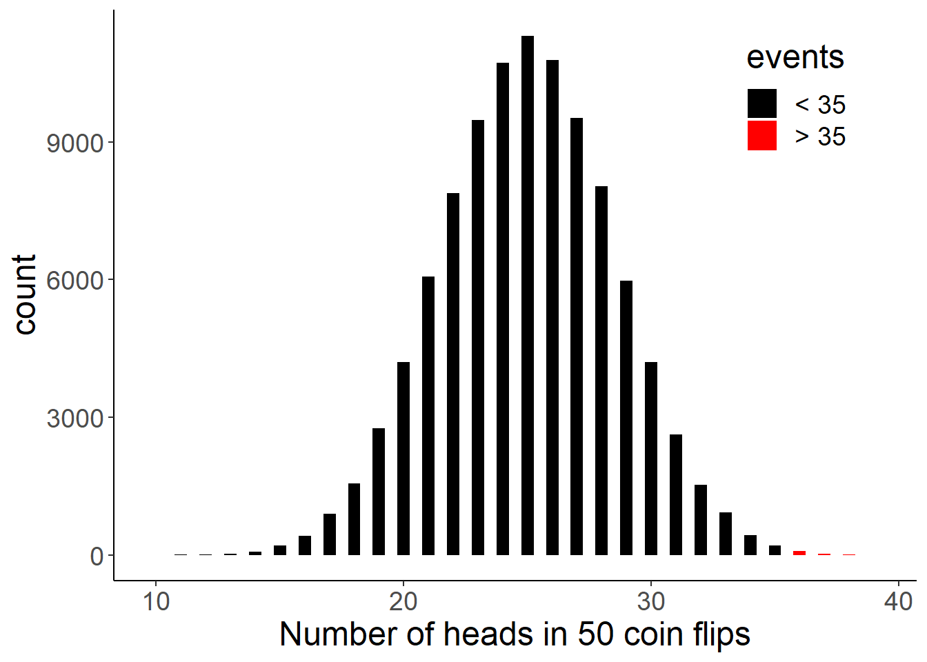
Binomial probability distributions help us to understand the likelihood of rare events and to set probable expected ranges.
The above plot illustrates if we randomly flip a coin 50 times, we will most likely get between 20 to 30 successes (heads) and events such as having more more than 35 successes (heads) out of 50 trials are very unlikely. The bars in red represents the sets which had 35 or more heads.
So what are all those will be useful for?
You can impress your friends with your ability to use binomial distributions to predict coin flipping outcomes, but let’s look at other real life applications of them.
- The performance of a machine learning model
You built a machine learning model with a binary outcome. Let’s say pathological image recognition algorithm for liver cancer that is 90% accurate. You tested 100 patients and you want to know your 95% confidence interval? Or your new results showed that your model detected less than 70 patients correctly. Is it possible? Or you should start optimizing your parameters again?
- Number of patients responding to a treatment.
Let’s say you have a new therapy for cancer which has 10% probability to cure a patient. You have 500 patients which took the drug. The expected number of recovering patients is 50. But in your trial 75 patients responded. Is this due to chance or a significant effect? Or you should start looking underlying factors if there is something about the therapy or the patient group?
- Think about a hospital emergency station.
You are a hospital manager and you want to organize the staff numbers correctly for different weekdays. You know total number of patients came in to a emergency station because of alcohol poisoning in a given time period. You can analyse the distribution of patient numbers for each day of the week. Most likely you will have more such cases in the weekends and you need larger staff.
This will be also true for other businesses. They can use binomial distributions to calculate changes in demand and plan accordingly.
- If you are running a Webserver.
You can allocate your resources better by identifying times when traffic will be higher.
Some other questions in which binomial distributions will come in handy are:
- Number of people who answered ‘yes’ to a survey question
- How many games a team will win in one season?
- Vote counts for a candidate in an election.
- Number of defective products in a production run.
Binomial distributions are common and they have many applications of real life situations.
We can expand binomial distributions to multinomial distributions when instead there are more than two outcomes for the single event.
Such as there are 6 outcomes when rolling a die, or analyzing distributions of eye color types (Black, blue, green etc) in a population. When it is about distributions for events with multiple categories think about multinomial distributions.
If the number of observations(n) are large we can think of a multinomial draw as being a series of binomial draws (Gentle, 2003, pp. 198–199). For example, when rolling a die the 6 categories can be thought of a combination of 6 different binomial trials (getting 1, 2 ,3 and so on).
If you are not convinced just by reading this, I will simulate how the shape of a multinomial event changes by increasing the number of trials.
Let’s use some real life data to apply our knowledge so far. The data comes from TidyTuesday which I introduced in my last post.
It contains data about Horror Movies released since 2012. And what I asked was whether horror movies are more likely be released at the 13th each month?
If you are in the right mindset anything feels better and if you are not in the mood nothing will make us happy. The mindset we have prior to an event influences what we will feel about an event. This is at least what behavioral scientist Robert Cialdini’s research says.
Imagine you are a horror movie fan and you went to the cinema. On the screen couple of ads are running just before the movie starts. You approach your mobile to turn off the voice and the date catches your attention, it is the 13th.
And usually with the number 13 we associate cursed events. Do you think it will influence your impression about the movie?
We don’t know if this is true but I wanted to test whether movie makers have similar ideas and selected 13th as the release date more often than other days. So, I explored Horror movies data and calculated number of releases in different days of the month.
Let’s look at the data.
horror_movies <- readr::read_csv("https://raw.githubusercontent.com/rfordatascience/tidytuesday/master/data/2019/2019-10-22/horror_movies.csv")

dim(horror_movies)
## [1] 3328 12head(horror_movies)## # A tibble: 6 x 12
## title genres release_date release_country movie_rating review_rating
## <chr> <chr> <chr> <chr> <chr> <dbl>
## 1 Gut ~ Drama~ 26-Oct-12 USA <NA> 3.9
## 2 The ~ Horror 13-Jan-17 USA <NA> NA
## 3 Slee~ Horror 21-Oct-17 Canada <NA> NA
## 4 Trea~ Comed~ 23-Apr-13 USA NOT RATED 3.7
## 5 Infi~ Crime~ 10-Apr-15 USA <NA> 5.8
## 6 In E~ Horro~ 2017 UK <NA> NA
## # ... with 6 more variables: movie_run_time <chr>, plot <chr>, cast <chr>,
## # language <chr>, filming_locations <chr>, budget <chr>I need some data pre-processing before I can make my visualizations. Dates are given in day:month:year format. I need to split them to individual columns. Also couple of movies do not have the day of the month. I will remove them.
horror_date <-  horror_movies %>%
                separate(
                  release_date,
                  c("day", "month", "year"),
                  sep = "-")

horror_date$day <- as.numeric(horror_date$day)

# Remove rows without Date of the month

horror_date <- horror_date %>% filter(day < 32)

# I am excluding Day 1 from the analysis (Most aggreements starts at 1st)

horror_date_table <- horror_date %>% filter(day > 1)

# Let's check what is the most common day in the month for a horror movie release
horror_date_table <-  horror_date_table %>%
  group_by(day) %>%
  count() %>%
  arrange(desc(n))
horror_date_table
## # A tibble: 30 x 2
## # Groups: day [30]
## day n
## <dbl> <int>
## 1 13 124
## 2 18 119
## 3 25 119
## 4 21 110
## 5 31 107
## 6 28 102
## 7 10 100
## 8 20 100
## 9 5 99
## 10 7 98
## # ... with 20 more rowsLet’s visualize.
# Final
horror_date_table$day <- as.character(horror_date_table$day)

my_title <- "Highest number of Horror movies are released at the 13th"

p <- horror_date_table %>%
    ungroup() %>%
    mutate(day=fct_reorder(day, n, .desc=TRUE)) %>%
    ggplot(aes(x=day, y=n)) +
    geom_col(aes(fill=n)) +
    scale_fill_viridis( direction =-1) +
    theme(
      plot.title = element_text(size=24, color= "black", hjust=0.5, vjust = -1),
      plot.subtitle = element_text(size=36, color= "red", hjust=0.5, vjust = -1),
      panel.background = element_rect(fill = "white"),
      plot.background = element_rect(fill = "white"),
      panel.grid = element_blank(),
      legend.position = "none",
      text = element_text(size=18),
      axis.text.x =element_text(vjust=12, size=17, colour= "white", face= "bold"),
      axis.title.x = element_text(vjust=9.5),
      axis.text.y=element_blank(),
      axis.ticks= element_blank(),
      plot.caption = element_text(hjust = 1, vjust = 10)) +
    labs(
          caption= "Source: IMDb, Plot: @dataatomic",
          x = "Day of the Month",
          y = "Number of movies released",
          title = my_title) +
    geom_label(aes(label = n), size=5, fill="yellow", alpha=0.9)
p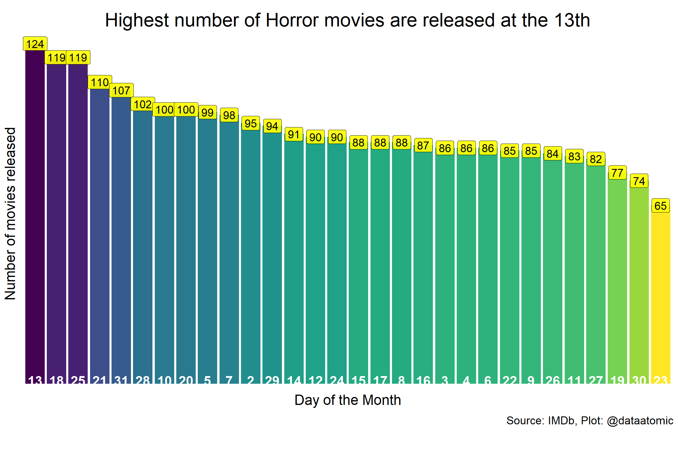
Is this significant?
In the data, there were 2782 movies associated with a release date. So expected movie release per day is 92 (2782 / 30).
This is a good example of a multinomial probability distribution with 30 categories, and since the number of samples are large it will approximate a binomial distribution.
Thus, we can apply binomial probability distributions for calculating the probabilities in our multinomial data.
We saw above that in some days more movies are released than the expected value. What we want to know is, which days are in the range of random chance and which days there is a significant preference or an aversion to release a movie.
# Size of our distribution is the total number of movies released
n_value <- horror_date_table %>% ungroup() %>% summarize(n2 = sum(n))
size <- n_value$n2
size
## [1] 2782# The probability (= success rate = a given outcome to occur = movie released)
p <- 1/30 # Since it can occur any of the 30 days in a monthsYou can simulate this 2782 movie release dates events 100.000 times with rbinom function and calculate the mean and variance.
# Simulated statistics

estimates <-  rbinom(100000, 2782, 1/30)

# Simulated mean
mean(estimates)
## [1] 92.73831# Simulated variance
var(estimates)## [1] 90.01739The average value is around 92 movies released in one day.
We can also calculate theoretical values by the derived mathematical formulas that define the binomial function:
Mean = size * p
Variance = size * p * (1 - p)
Let’s calculate.
# Theoretical statistics

# Expected mean = size * p
mean_theoretical <- 2782 * 1/30
mean_theoretical
## [1] 92.73333# Expected Variance = size * p * (1-p)
var_theoretical <- size * 1/30 * (1-1/30)
var_theoretical## [1] 89.64222Great, simulated and theoretical values are almost the same. So, I can use my simulations to find out 95% confidence interval which will contain the values that can happen due to random chance.
I will define an interval that contains 95% of probabilities in our simulated distributions. And the values outside will be the ones which were not due to random chance. To do this I need 2.5th and 97.5th quantiles of the distribution.
We can do this by the qbinom() function in r. For example qbinom(0.975, size, p) will return the value which will define the cut off which contains 0.975 of the probabilities. And our confidence interval will be the interval between:
qbinom(0.025, size, p) < Confidence Interval < qbinom(0.975, size, p)
# Boundaries for p values smaller than 0.05

lower <- qbinom(0.975, 2782, 1/30)
lower
## [1] 112upper <- qbinom(0.025, 2782, 1/30)
upper## [1] 75movies <- rbinom(100000, 2782, 1/30)
movies <- data.frame(movies)
movies <- movies %>% mutate(events = ifelse(movies > qbinom(.025, 2782, 1/30) & movies < qbinom(.975, 2782, 1/30), "95% Conf. Int.", "significant"))
movies %>% ggplot(aes(x=movies, fill = events)) +
geom_histogram(binwidth = 0.5) +
scale_fill_manual(values = c("black", "red")) +
theme_classic() +
theme(text = element_text(size = 18),
legend.position = c(0.85, 0.85)) +
labs(x = "Number of movie releases in a day")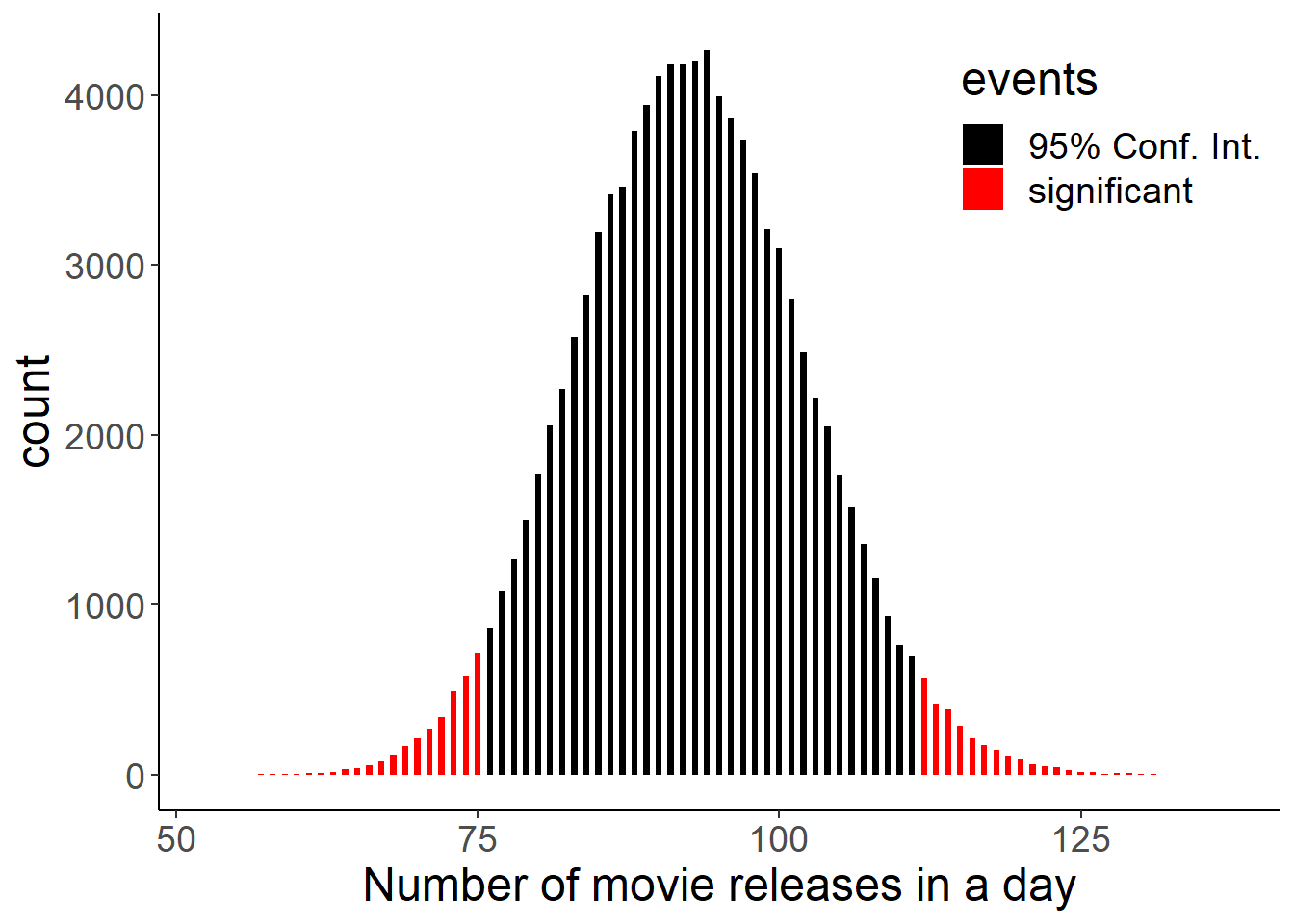
95% of the time, a specific day of month will have between 75 and 112 movie releases. Higher or lower values than this range can not happen due to random chance according to our probability distribution.
124 movies released at the 13th of any month. This value is above the 97.5th quantile. So it is significant. But what is the exact p value? Let’s define p value first.
How to calculate the p-value for a binomial test using pbinom?
For example in coin flipping, probability of heads is (0.5). If we follow our definition, p value is the sum of the probability of that event (0.5) and similar events which is equally or less likely i.e. tails (0.5). This makes our p value 0.5 + 0.5 = 1.
Similarly, in our horror movie data this will be the sum of the probabilities of getting 124 movie releases or events that are equally probable or rarer.
In R, pbinom function defines the cumulative probabilities. For example, pbinom(124, 2782, 1/30) will give us the cumulative probabilities of any number of movie releases up to 124. By using 1-pbinom(124, 2782, 1/30) we can find the sum of the probabilities with equal or lower chance than having 124.
Thus, p value for getting at least 124 movie release is;
# Probability of getting at least 124 movie releases (e.g. the 13th)

p_val_binom <- 2 * (1 - pbinom(124, 2782, 1/30))
p_val_binom
## [1] 0.001335455We multiplied by two because same rare events can happen in the left side of our confidence interval as well.
Let’s put those p values on our barplot to highlight the significant days.
# I will add a new column so I can separately define values outside the 95% confidence interval.

horror_date_table <- horror_date_table %>%
                     mutate(p_val = 2 * (1 - pbinom(n, 2782, 1/30,
                            lower.tail = ifelse(n>93, TRUE, FALSE)))) %>%
                     mutate(p_val = cut(p_val, breaks = c(-Inf, 0.001, 0.01, 0.05, Inf),
                                        labels = c("< 0.001","< 0.01", "< 0.05", "NS")))

# Visualize the significant days
p_ci <- horror_date_table %>%
    ungroup() %>%
    mutate(day=fct_reorder(day, n, .desc=TRUE)) %>%
    ggplot(aes(x=day, y=n)) +
    geom_col(aes(fill=p_val)) +
    scale_fill_manual(values = viridis(4))  +
    theme(
        plot.title = element_text(size=24, color= "black", hjust=0.5, vjust = -1),
        plot.subtitle = element_text(size=36, color= "red", hjust=0.5, vjust = -1),
        panel.background = element_rect(fill = "white"),
        plot.background = element_rect(fill = "white"),
        panel.grid = element_blank(),
        text = element_text(size=18),
        axis.text.x =element_text(vjust=12, size=17, colour= "white", face= "bold"),
        axis.title.x = element_text(vjust=9.5),
        axis.text.y=element_blank(),
        axis.ticks= element_blank(),
        plot.caption = element_text(hjust = 1, vjust = 10)) +
    labs(
        caption= "",
        x = "Day of the Month",
        y = "Number of movies released",
        title = "Calculating p values in binomial distributions") +
    geom_label(aes(label = n), size=5, fill="yellow", alpha=0.9)
p_ci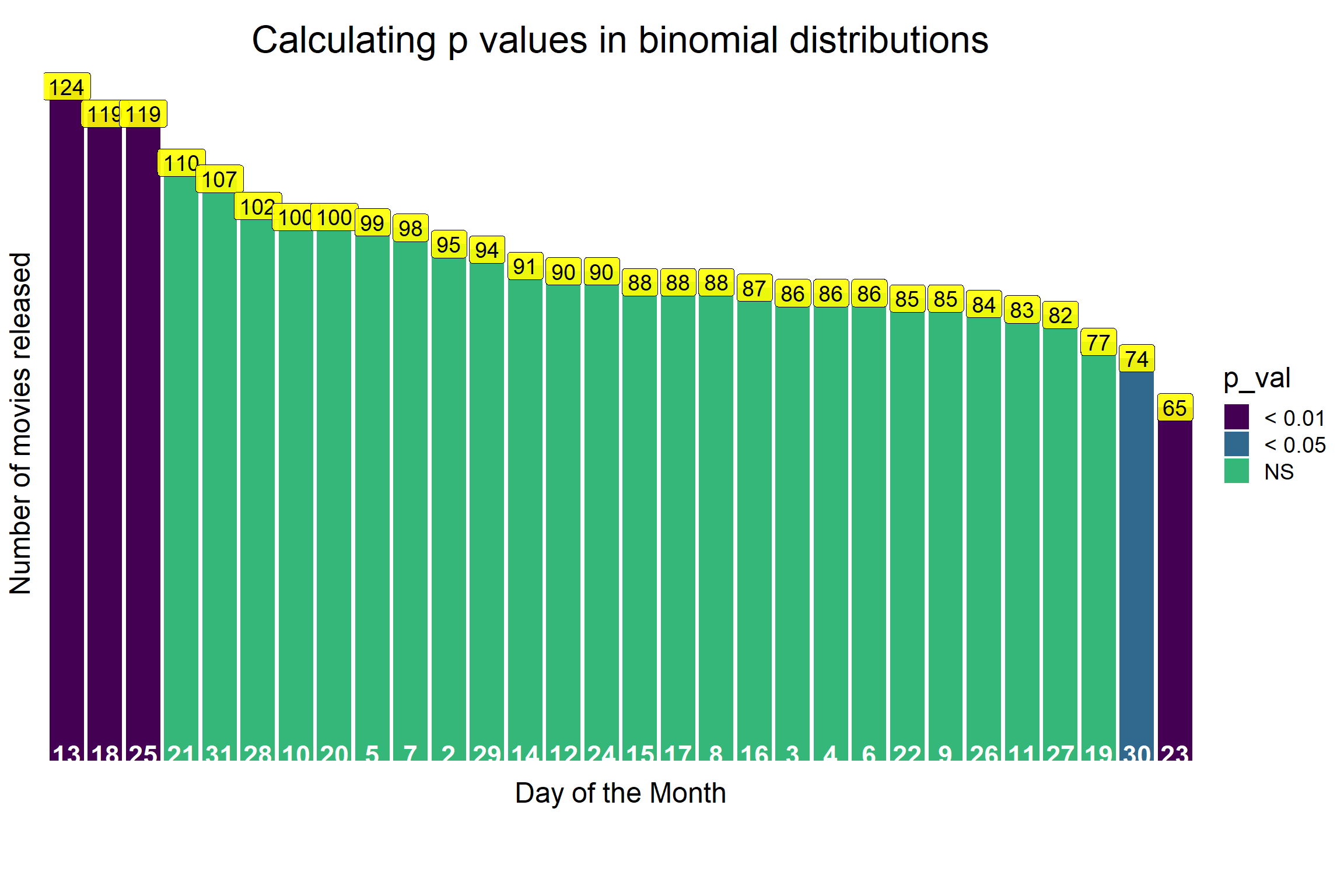
We tested our hypothesis about movie makers and calculated the p value and used the pbinom() function and found couple of other days where movies are more or less likely to be released.
However, another widely used way to calculate p values is to calculate the mean of the distribution and its standard deviation and to verify how many standard deviations the observed value is away from the mean (the z score).
Calculating the p-value by normal approximation
When the sample size is large, binomial distributions can be approximated by a normal distribution. To build the normal distribution, I need mean and standard deviation. I can calculate this from the horror movie data.
sample_mean <- horror_date_table %>% ungroup() %>% summarise(n=mean(n))
sample_mean
## # A tibble: 1 x 1
## n
## <dbl>
## 1 92.7p <- 1/30
sample_variance <- 2782 * p * (1-p)
sample_variance## [1] 89.64222sample_sd <- sqrt(sample_variance)
sample_sd## [1] 9.467958I can calculate the z-score for our observation of 124 movies that are released on the 13th. Simply, z-score is: how many standard deviations an observation is away from the mean. Since 95% of the observations will fall within 1.96 standard deviations from the mean in a normal distribution, a higher z-score will show that our p value is indeed significant.
# Calculate z-score for observation 13th of the month = 124 movies are
# released
observation <- 124
z_score <- (observation - sample_mean) / sample_sd
z_score
## n
## 1 3.302367I can calculate the exact p value by using a normal distribution function pnorm() and the z score we found.
# Calculate the p-value of observing 124 or more movie releases in a day

p_val_nor <- 2 * pnorm(3.302, lower.tail = FALSE)
p_val_nor
## [1] 0.0009599807As expected, I found similar values (Normal: 0.00095, Binomial: 0.00133) by using an approximation of a normal distribution and by using binomial distributions. Both methods proves that Horror movies are more likely to be released at the 13th.
Future thoughts / Conclusions
Many events in real life can be explained by binomial probability distributions, and they allow us to calculate whether or not the events happened due to random chance and test our hypotheses.
It can be a fun data analysis such as in horror movies, or more serious subjects like testing of new medicines or predicting accuracy of machine learning algorithms detecting diseases.
Until next time!
Serdar
Serdar Korur
Data Scientist and PhD in Molecular Biology
Serdar is a Data Scientist and PhD in Cell Biology