Speed boosting in R: Writing efficient code & parallel programming
Have more things happen at once: Parallel Programming
Parallel processing is about using multiple cores of your computer’s CPU to run multiple tasks simultaneously. This enables you to complete the same task multiple times quicker!
In R, usually computations run sequentially. When we initiate multiple tasks they are performed one after the other, new task starts only after the previous one is completed.
This might become the bottleneck when you come across a computationally heavy process. Such as running monte carlo simulations or fitting multiple machine learning models.Typically, if I have a process which runs longer than 3 minutes, I consider using parallel processing.
It might sound complicated but parallel computing is simple. When you have a repetitive task which takes too much of your valuable time why not implement it and save time? Even if you have a single task, you can benefit from parallel processing by dividing the task into smaller pieces.
Two widely used packages for parallel processing are parallel and foreach.
Let’s do some parallel processing..
What is our goal?
I recently analyzed data from horror movies released in the world between 2012 and 2017. What caught my attention was that movies are more likely to be released at the 13th of each month. You can visit my recent post if you want to know more about this data.
Let’s get the data
There are 2782 movies released in one of the 30 days (categories). The resulting table below shows the days of the month and how many movies released at that day.
library(tidyverse) # ggplot2, dplyr, tidyr, readr,
                   # purrr, tibble, stringr, forcats
horror_movies <- readr::read_csv("https://raw.githubusercontent.com/rfordatascience/tidytuesday/master/data/2019/2019-10-22/horror_movies.csv")
dim(horror_movies)## [1] 3328 12horror_date <- horror_movies %>%
separate(
release_date,
c("day", "month", "year"),
sep = "-")
horror_date$day <- as.numeric(horror_date$day)
# Remove rows without Date of the month
horror_date <- horror_date %>% filter(day < 32)
# I am excluding Day 1 from the analysis (Most aggreements starts at 1st)
horror_date_table <- horror_date %>% filter(day > 1)
# let's check what is the most common day in the month for a horror movie release
data <- horror_date_table %>%
group_by(day) %>%
count() %>%
arrange(desc(n))
data %>% print(n=30)## # A tibble: 30 x 2
## # Groups: day [30]
## day n
## <dbl> <int>
## 1 13 124
## 2 18 119
## 3 25 119
## 4 21 110
## 5 31 107
## 6 28 102
## 7 10 100
## 8 20 100
## 9 5 99
## 10 7 98
## 11 2 95
## 12 29 94
## 13 14 91
## 14 12 90
## 15 24 90
## 16 8 88
## 17 15 88
## 18 17 88
## 19 16 87
## 20 3 86
## 21 4 86
## 22 6 86
## 23 9 85
## 24 22 85
## 25 26 84
## 26 11 83
## 27 27 82
## 28 19 77
## 29 30 74
## 30 23 65I will simulate 1 million multinomial trials of distributing 2782 movies to 30 days of the month. This type of distributions (k > 2) are called multinomial distributions.xx`
I created a function to find p values for each day. But it takes sometime to run. I will try to improve the runtime by optimizing my code and using parallel processing.
multfun <- function(x){
  a <- list()
  avc <- rmultinom(1000000, size=2782, prob=rep(1/30, 30))  # Create probability matrix
  for (i in 1:30){ a[[i]] <- mean(avc[i,1:1000000] >=x) }   # Find probabilities for each day
  ifelse(do.call(sum,a)/30 <= 0.5, p_val <-  2 * do.call(sum,a)/30,
                                   p_val <- 2*(1 - do.call(sum,a)/30))
}
multfun() uses rmultinom() function to produce a matrix of monte carlo simulations of 1.000.000 random multinomial distributions with 30 categories. Then calculates total probabilities of any given observation or rarer events at each day from this matrix.
This actually translates into the p value for a given (n) observation. For example, when I run multfun(124), It will give me the p value for observing a day with at least 124 movie releases.
# Run an example
multfun(124)
## [1] 0.001844267To calculate the p values for the top 5 days with highest number of movie releases, I can run multfun() multiple times for each value.
Execute the multfun() function multiple times
system.time({
multfun(124)
multfun(119)
multfun(110)
multfun(107)
multfun(102)
})
## user system elapsed
## 15.72 0.21 15.94For few values it can be ok, but easier methods exist if you need to run your function repetitvely for a bigger number of inputs.
Using lapply() function
Instead of running a function for different input values several times, you can use lapply() function. It loops over a given vector or list input (l in lapply comes from list), and applies the input function to each element in that list.
system.time({
lapply(c(124,119,119,197,102), multfun)
})
## user system elapsed
## 15.64 0.29 15.92Using parallel package functions: parLapply()
If you have ever used any of lapply() or sapply function you are halfway in parallel processing.
Preparation for parallel processing
You can use detectCores() function to find out how many cores are available in your CPU.
Then, to create the clusters required apply makeCluster() with the number of cores you intend to use. In my computer, I have 6 cores and I will assign 5 cores as the multiple workers.
Parallel processing: parLapply
parLapply is the easiest way to parallelise computation. You first need to replace lapply with parLapply and enter an extra cluster argument.
Then, an additional preparation step to create the clusters required. makeCluster() function creates the number of cluster that you intend to use. In my computer, I have 6 cores and I will assign 5 cores as the multiple workers.
library(parallel)
system.time({
n_cores <- detectCores(logical=FALSE)
cl <- makeCluster(n_cores-1)
parLapply(cl , c(124,119,119,197,102), multfun)
})
## user system elapsed
## 0.02 0.01 4.54stopCluster(cl)When done, include stopCluster() argument to avoid running R sessions in different clusters in the background.
Theoretically, I can expect 5X quicker processing with 5 cores. But there are overhead costs. Additional preparation steps such as makecluster() function also takes time.
We had much quicker execution by parallel processing. Is there a room for further improvement?
Let’s look at our multfun function again…
multfun <- function(x){
  a <- list()
  avc <- rmultinom(1000000, size=2782, prob=rep(1/30, 30))  # Create probability matrix
  for (i in 1:30){ a[[i]] <- mean(avc[i,1:1000000] >=x) }   # Find probabilities for each day
  ifelse(do.call(sum,a)/30 <= 0.5, p_val <-  2 * do.call(sum,a)/30,
                                   p_val <- 2*(1 - do.call(sum,a)/30))
                       }
In R, it is possible to do things in multiple ways. Sometimes we need more readable version and sometimes just fast code. I see that multfun uses a list and a for loop. If I find a way without using them I can get a faster run.
Improved multfun: Define the function without using a loop and list
Mean function in R can be vectorized instead of looping.
I can achieve the same result what the first multfun() was doing by including what for loop was doing inside the “[ ]”. Mean function will be applied find the total proportion of values equal or bigger than x.
multfun_opt <- function(x){
  avc <- rmultinom(1000000, size=2782, rep(1/30, 30))
  p <- mean(avc[1:30, 1:1000000] >=x)
  ifelse(p <= 0.5, p_val <-  2 * p, p_val <- 2*(1 - p))}
Let’s check whether improved multfun is faster.
system.time({
n_cores <- detectCores(logical=FALSE)
cl <- makeCluster(n_cores-1)
parLapply(cl , c(124,119,119,197,102), multfun_opt)
})
## user system elapsed
## 0.00 0.06 4.32stopCluster(cl)Since rmultinom is the bottleneck here, we did not see very big improvement in overall function. We got 10-20% improvement. But it is good to know, what we can improve when we really need it.
Let’s compare only the part of the function which uses the vectorized operation and the one with for loop.
avc <- rmultinom(1000000, size=2782, prob=rep(1/30, 30))
a <- list()

system.time({
  for (i in 1:30){ a[[i]] <- mean(avc[i,1:1000000] >=124) }
  ifelse(do.call(sum,a)/30 <= 0.5, p_val <-  2 * do.call(sum,a)/30,
                                   p_val <- 2*(1 - do.call(sum,a)/30)) })
## user system elapsed
## 0.41 0.01 0.42system.time({
p <- mean(avc[1:30, 1:1000000] >=124)
ifelse(p <= 0.5, p_val <- 2 * p, p_val <- 2*(1 - p)) })## user system elapsed
## 0.22 0.02 0.24Vectorised version is twice faster!!
Further Improvement
You can use Rprof() function to profile your process, it will return how much time each subprocess takes time. Let’s profile our function.
multfun_opt <- function(x){
  avc <- rmultinom(1000000, size=2782, rep(1/30, 30))
  p <- mean(avc[1:30, 1:1000000] >=x)
  ifelse(p <= 0.5, p_val <-  2 * p, p_val <- 2*(1 - p))
  }

Rprof()
multfun_opt(124)
## [1] 0.0018542Rprof(NULL)
summaryRprof()$by.self## self.time self.pct total.time total.pct
## "rmultinom" 1.80 93.75 1.80 93.75
## ">=" 0.08 4.17 0.08 4.17
## "mean" 0.02 1.04 0.12 6.25
## "mean.default" 0.02 1.04 0.02 1.04In profile summary, total.pct shows the total percentage of the duration of each task inside the function. We can see that rmultinom() part of takes more than 90% of the processing time.
If we are looking further improvement we can focus on it. To improve rmultinom() part, I will isolate it by splitting the multfun into two functions.
Above, first improvement was using parLapply instead of lapply and second replacing a loop with a faster vectorized operation. Now, we will utilize another approach, dividing a task into smaller pieces.
I need to create a new rmultinom() function, which I call fastbinom. To keep things simple, it will take only one argument which I will use to divide 1.000.000 rmultinom simulations into 5 equal parts of 200.000 rmultinom simulations. Each will be handled by a different core in my CPU boosting my speed.
fastbinom <- function(x) {
  rmultinom(x, size=2782, rep(1/30,30))
}

multfun_fin <- function(x){
  p <- mean(avc[1:30, 1:1000000] >=x)
  ifelse(p <= 0.5, p_val <-  2 * p, p_val <- 2*(1 - p))
}
Here comes an additional overhead. Since, multfun_fin will be executed on different cores, we need to export the data to each cluster. Windows rely on clusterExport() for data to be copied to each cluster.
Test the final optimized code.
# Final optimized code
system.time({
cl <- makeCluster(5)
avc <- parLapply(cl , c(200000, 200000, 200000, 200000, 200000), fastbinom)
avc <- do.call(cbind, avc)
clusterExport(cl, varlist="avc", envir=environment())
parLapply(cl, c(124,119,119,197,102), multfun_fin)
})
## user system elapsed
## 0.60 0.61 3.05stopCluster(cl)Quite a bit improvement!
Final test
Let’s now put things together, I will test different versions I created so far. But this time for more input values, I will use my function for each of the 30 categories and by using up to 1.000.000 simulations.
Let’s call the initial version: original, second parLapply, third parLapply, optimized and the last parLapply/fastbinom
multfun <- function(x){
  a <- list()
  avc <- rmultinom(1000000, size=2782, prob=rep(1/30, 30))  # Create probability matrix
  for (i in 1:30){ a[[i]] <- mean(avc[i,1:1000000] >=x) }   # Find probabilities for each day
  ifelse(do.call(sum,a)/30 <= 0.5, p_val <-  2 * do.call(sum,a)/30,
                                   p_val <- 2 * (1 - do.call(sum,a)/30))
}


# Original
system.time({
lapply(data$n, multfun)
})
## user system elapsed
## 92.37 1.43 93.82# parLapply
system.time({
n_cores <- detectCores(logical=FALSE)
cl <- makeCluster(n_cores-1)
parLapply(cl , data$n, multfun)
})## user system elapsed
## 0.03 0.03 24.97stopCluster(cl)
multfun_opt <- function(x){
avc <- rmultinom(1000000, size=2782, rep(1/30, 30))
p <- mean(avc[1:30, 1:1000000] >=x)
ifelse(p <= 0.5, p_val <- 2 * p, p_val <- 2*(1 - p))
}
# parLapply, optimized
system.time({
n_cores <- detectCores(logical=FALSE)
cl <- makeCluster(n_cores-1)
parLapply(cl , data$n, multfun_opt)
})## user system elapsed
## 0.00 0.03 21.75stopCluster(cl)
multfun_fin <- function(x){
p <- mean(avc[1:30, 1:1000000] >=x)
ifelse(p <= 0.5, p_val <- 2 * p, p_val <- 2*(1 - p))
}
# parLapply, fastbinom
system.time({
cl <- makeCluster(5)
avc <- parLapply(cl , c(200000, 200000, 200000, 200000, 200000), fastbinom)
avc <- do.call(cbind,avc)
clusterExport(cl, varlist="avc", envir=environment())
parLapply(cl, data$n, multfun_fin)
})## user system elapsed
## 0.56 0.60 4.10stopCluster(cl)Here is an additonal comparision, testing time differences between different versions and to be more precise I simulated up to 10.000.000 multinomial distributions.
library(readxl)
library(tidyverse)
library(viridis)
## Loading required package: viridisLitespeedtest <- read_excel("posts_data/parallelprocessing_speed_tests.xlsx", sheet =3)## New names:
## * `` -> ...1speedtest <- speedtest[-1]
spd <- gather(speedtest, version, seconds, -c(rmultinom,n))
spd$version <- factor(spd$version, labels = c("original", "parlapply", "parLapply/opt", "parLapply/fastbinom"))
spdplot <- spd %>% filter(n >5) %>%
ggplot(aes(x=rmultinom, y=seconds, color=version)) +
geom_line() +
theme(text = element_text(size=18)) +
labs( x = "Number of simulations",
y = "Time (seconds)")spdplot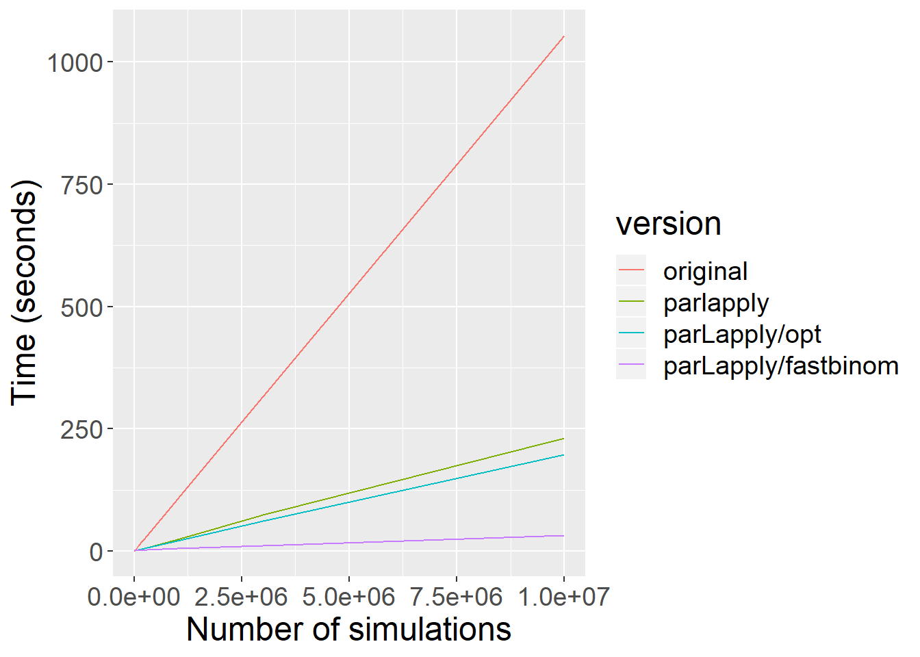
spd %>% filter(rmultinom ==10000000, n >5) %>%
  ggplot(aes(x=version, y=seconds)) + geom_col() +
  theme(text = element_text(size=15)) +
  geom_label(aes(label = seconds), alpha = 0.5)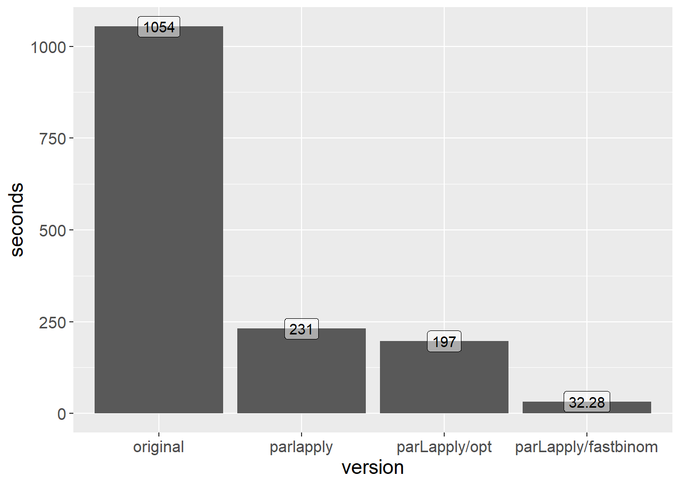
By splitting our original function into two and then applying parallel processing for each subtask we achieved more than 30X speed gain.
Summary
Parallel processing is easy and can get your tasks extremely faster.
Until next time!
Serdar
Serdar Korur
Data Scientist and PhD in Molecular Biology
Serdar is a Data Scientist and PhD in Cell Biology