Genomics at superresolution: Mapping Drug targets on single cell resolution in Fibrosis
Advances in microfluidic technologies enabled us to barcode single cells in lipid droplets and to resolve genomes of individual cells from a sequencing mixture (e.g, 10X Genomics). By using Single cell RNA sequencing (scRNA-seq) we can discover rare cell populations and genes that are specifically acting in those. Potential is high and the list of publications growing daily.
- If you are a scientist in a biotech exploring novel targets those might be a great source to gather specific information.
Seurat package is a great tool for digging into single cell datasets. It will open you access beyond what is in the publications. You can find many tutorials in their website.
Here, I will focus on a recent paper which explored transcriptome of lung cells from Pulmonary fibrosis patients by scRNAseq.
- Pulmonary fibrosis is a progressive scarring of the lung tissue leading to death within 3-4 years.
- Current therapies do not increase the survival
- Many Biotech companies are developing novel drugs
Our workflow will be in three steps
- Basic Seurat workflow
- Identify cell types on a tSNE plot
- Visualize drug targets on single cell plots
I picked up scRNA-seq data from a patient with Polymyositis associated interstitial lung disease.
—> Download Single Cell RNA seq data
Seurat Workflow
Load the packages that will be used.
library(Seurat)
library(dplyr)
library(ggplot2)
Importing the h5 file
Here the data comes as an h5 file. But no worries, we can handle that with Read10X_h5 function in Seurat. Since the file is directly under my working directory I can apply Read10X_h5("Filename.h5")
MyoILD_01 <- Read10X_h5("posts_data/GSM3489196_Myositis-ILD_01_filtered_gene_bc_matrices_h5.h5")
Fib <- CreateSeuratObject(counts = MyoILD_01, min.cells = 3, project= "FightFibrosis", min.features = 200)
Fib
## An object of class Seurat
## 20246 features across 7163 samples within 1 assay
## Active assay: RNA (20246 features)Our Data matrix now contains 20246 genes and 7163 cells
A Quick look at the raw count data
# Lets examine a few genes in the first thirty cells
MyoILD_01[c("SPP1","TGFB1","CCL2"), 1:30]
## 3 x 30 sparse Matrix of class "dgCMatrix"
##
## SPP1 1 . . 2 . . . 33 . . 1 . . . . . . . . . . . . . . . 9 . . 20
## TGFB1 . . . . 1 . . . . . . . . . 1 . 3 . . . . . . . 1 2 . . . .
## CCL2 5 . . 2 . . . . . . . . . . . . . . . . . . . . . . . . . .Standard pre-processing workflow for scRNA-seq data
Pre-processing involves filtration of cells based on Quality control metrics (e.g .mitochondrial contamination, Coverage). We will proceed by normalization and identification of the highly variable features then at the end we will scale the data.
QC and selecting cells for further analysis
# Let's add Mitochondrial stats to Fib data. [[ operator can add
# columns to object metadata.

Fib[["percent.mt"]] <- PercentageFeatureSet(object = Fib, pattern = "^MT-")
# Quick look at the Quality control metrics for the first 5 cells
head(x = Fib@meta.data, 5)## orig.ident nCount_RNA nFeature_RNA percent.mt
## AAACCTGAGATCCCGC-1 FightFibrosis 2257 1010 4.386354
## AAACCTGAGCAGCCTC-1 FightFibrosis 3367 713 66.914167
## AAACCTGAGCCAGAAC-1 FightFibrosis 7354 1943 3.929834
## AAACCTGAGGGATGGG-1 FightFibrosis 9323 2786 8.430763
## AAACCTGAGTCGTACT-1 FightFibrosis 2937 1125 6.775621Violin plots to visualize QC metrics
#Visualize QC metrics as a violin plot
VlnPlot(object = Fib, features = c("nFeature_RNA", "nCount_RNA", "percent.mt"),
        ncol = 3)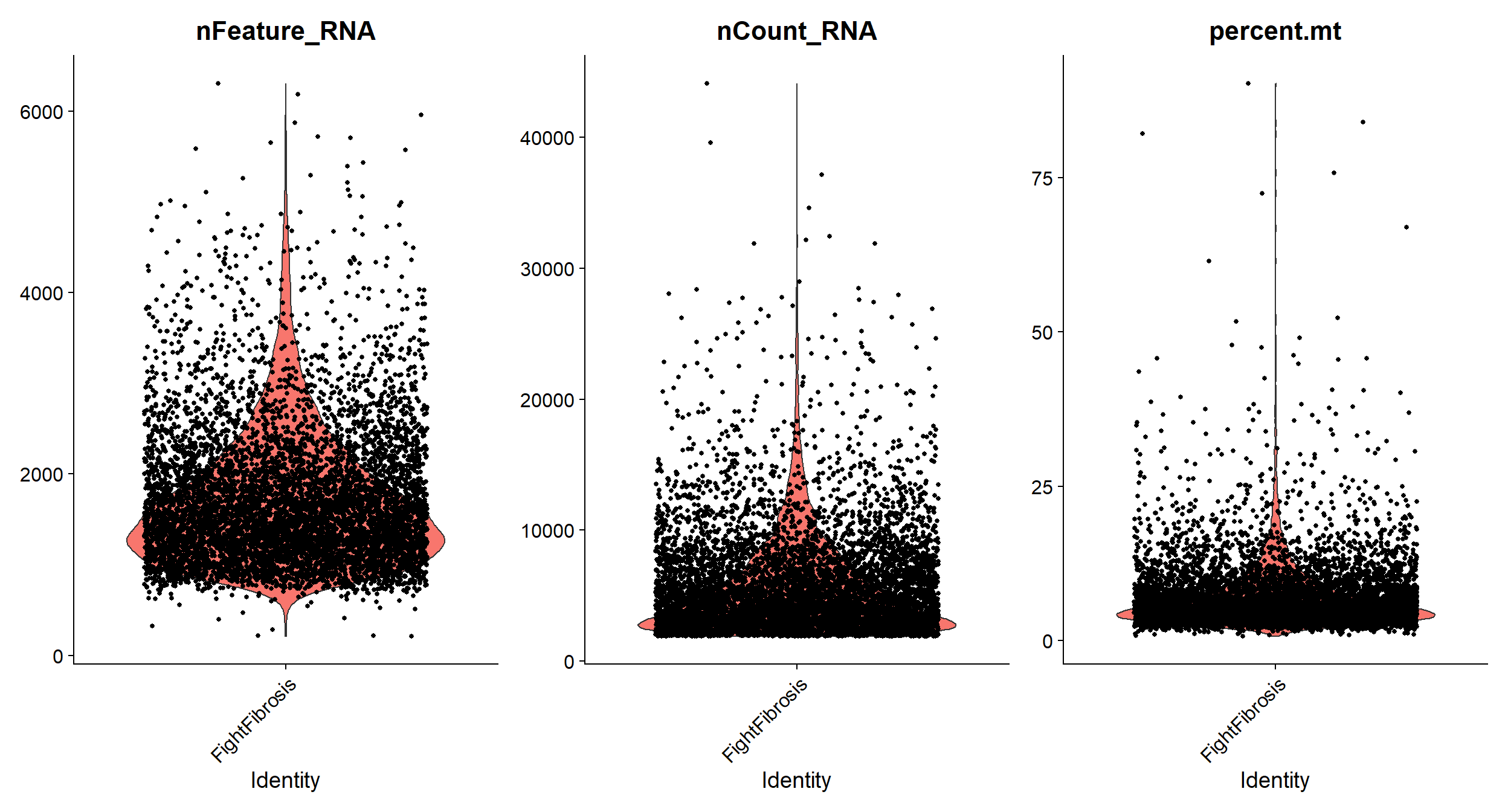
# We will use FeatureScatter to visualize feature-feature relationships like
# RNA counts or percentage of mitochondiral contamination

plot1 <- FeatureScatter(object = Fib, feature1 = "nCount_RNA", feature2 = "percent.mt")
plot2 <- FeatureScatter(object = Fib, feature1 = "nCount_RNA", feature2 = "nFeature_RNA")
CombinePlots(plots = list(plot1,plot2))
## Warning: CombinePlots is being deprecated. Plots should now be combined using
## the patchwork system.
# As you see on the left plot cells with high percentage of mitochondrial genes
# have very low numbers of RNA indicating that they are low quality/dead cells.
# Let's remove them.
Fib <- subset(x = Fib, subset = nFeature_RNA > 200 & nFeature_RNA < 4000 &
              percent.mt < 12.5)
Normalize the data
Log normalization helps to reduce the influences of the outliers.
Normalized values will be stored in Fib[["RNA"]]@data.
Fib <- NormalizeData(object = Fib, normalization.method = "LogNormalize",
                     scale.factor = 1e4)
Identify highly variable features
Let’s calculate the features that exhibit high cell-to-cell variation in the dataset. Focusing on those genes will help to highlight biological signal.
Fib <- FindVariableFeatures(object = Fib, selection.method = 'vst',  nfeatures = 2000)

# Identify the 10 most highly variable genes
top10 <- head(x = VariableFeatures(object = Fib), 10)
top10
## [1] "SCGB1A1" "SCGB3A1" "SFTPC" "SCGB3A2" "HBB" "PLA2G2A" "MT1G"
## [8] "TPSB2" "FABP4" "MT1H"# Plot variable features with and without labels
plot1 <- VariableFeaturePlot(object = Fib)
plot2 <- LabelPoints(plot = plot1, points = top10, repel = TRUE)
CombinePlots(plots = list(plot1, plot2))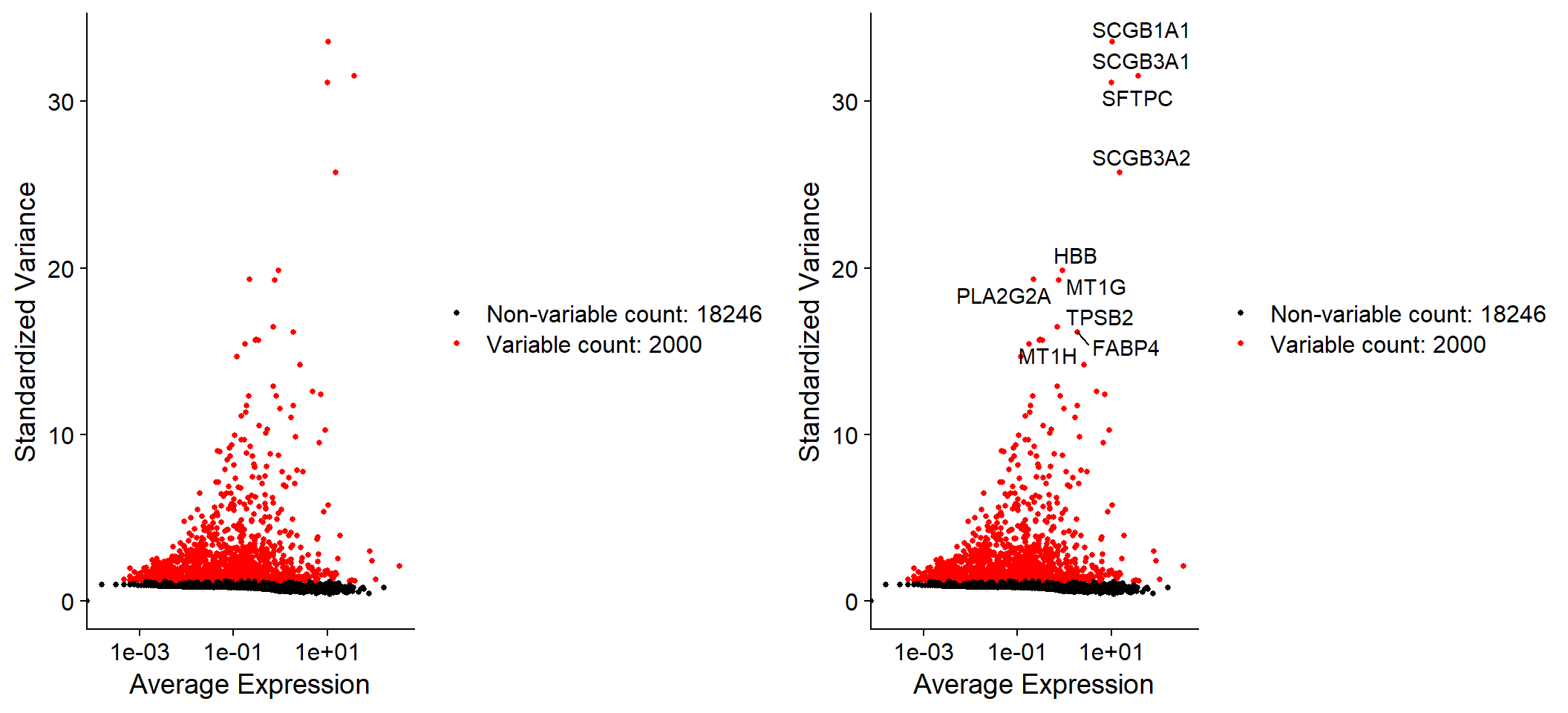
Scale the data
Next, apply a linear transformation that is a standard pre-processing step prior to dimensional reduction techniques like PCA. The ScaleData function:
Highly-expressed genes might dominate downstream analyses since their expression range is much higher than most other genes. In order to prevent this we need to;
- shift the expression of each gene, so that the mean expression across cells is 0
- scale the expression of each gene, so that the variance across cells is;
Apply the ScaleData function
all.genes <- rownames(x = Fib)
Fib <- ScaleData(object = Fib, features = all.genes)
# Another factor that can influence downstream analyses is cell cycle status,
# cells that arenormally cycling but in different phases of cell cycle # might appear as separate populations.
# Seurat is preloaded with list of cell cycle markers, from Tirosh et al. 2015,
# segregate this list into markers of G2/M phase and markers of S phase
s.genes <- cc.genes$s.genes
g2m.genes <- cc.genes$g2m.genes
Fib <- CellCycleScoring(Fib, s.features = s.genes, g2m.features = g2m.genes, set.ident = TRUE)
# We can view cell cycle scores and phase assignments with
head(Fib[[]])## orig.ident nCount_RNA nFeature_RNA percent.mt
## AAACCTGAGATCCCGC-1 FightFibrosis 2257 1010 4.386354
## AAACCTGAGCCAGAAC-1 FightFibrosis 7354 1943 3.929834
## AAACCTGAGGGATGGG-1 FightFibrosis 9323 2786 8.430763
## AAACCTGAGTCGTACT-1 FightFibrosis 2937 1125 6.775621
## AAACCTGAGTCGTTTG-1 FightFibrosis 5447 1719 4.149073
## AAACCTGCAAGTCTAC-1 FightFibrosis 6453 1836 2.773904
## S.Score G2M.Score Phase old.ident
## AAACCTGAGATCCCGC-1 0.006739441 -0.016659228 S FightFibrosis
## AAACCTGAGCCAGAAC-1 -0.040762255 -0.010151464 G1 FightFibrosis
## AAACCTGAGGGATGGG-1 -0.048223904 -0.025580453 G1 FightFibrosis
## AAACCTGAGTCGTACT-1 0.076114887 0.009717348 S FightFibrosis
## AAACCTGAGTCGTTTG-1 -0.045171005 -0.053868788 G1 FightFibrosis
## AAACCTGCAAGTCTAC-1 0.003354484 -0.009033119 S FightFibrosis# Regress out cell cycle scores during data scaling
Fib <- ScaleData(Fib, vars.to.regress =
c("S.Score", "G2M.Score"), features =rownames(Fib))Perform linear dimensional reduction
Each gene creates another dimension in our dataset, but most of those do not play a role in differentiating subgroups of cells. Principal components analyses (PCA) helps us by reducing the dimensions of our data into components which explains most of the variation.
Fib <- RunPCA(object = Fib, features = VariableFeatures(object = Fib),
              ndims.print = 10, nfeatures.print = 10)
## PC_ 10
## Positive: VCAN, MCEMP1, S100A8, FCN1, CD2, IL32, S100A6, TIMP1, CCL5, CD3D
## Negative: CHIT1, A2M, CHCHD6, AC079767.4, SEPP1, ALOX15B, GPNMB, DNASE2B, LIPA, SLC40A1Visualize the PCA results
# Examine and visualize PCA results a few different ways
print(x = Fib[['pca']], dims = 1:5, nfeatures = 5)
## PC_ 1
## Positive: TMSB4X, TYROBP, FTL, FCER1G, VIM
## Negative: RSPH1, C9orf24, TMEM190, C20orf85, FAM183A
## PC_ 2
## Positive: FTH1, CTSS, TYROBP, B2M, FCER1G
## Negative: GPRC5A, SFTPB, CEACAM6, HOPX, MUC1
## PC_ 3
## Positive: PLA2G2A, GFPT2, MEDAG, COL3A1, COL1A2
## Negative: SFTPB, SFTPA2, SFTA2, SFTPA1, SLC34A2
## PC_ 4
## Positive: SFTPC, NAPSA, SFTPD, LRRK2, LAMP3
## Negative: S100A2, KRT19, KRT5, AKR1C1, BPIFB1
## PC_ 5
## Positive: CPA3, TPSAB1, TPSB2, MS4A2, GATA2
## Negative: S100A6, CSTB, S100A10, GCHFR, TXNVizDimLoadings(object = Fib, dims = 1:2, reduction = 'pca')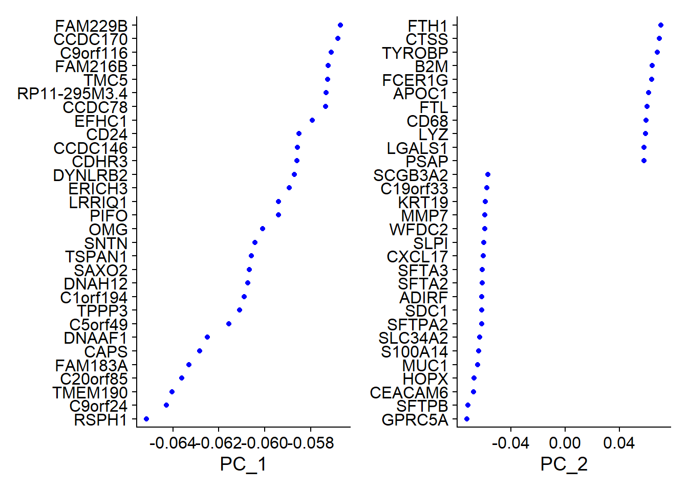
DimPlot(object = Fib, reduction = 'pca')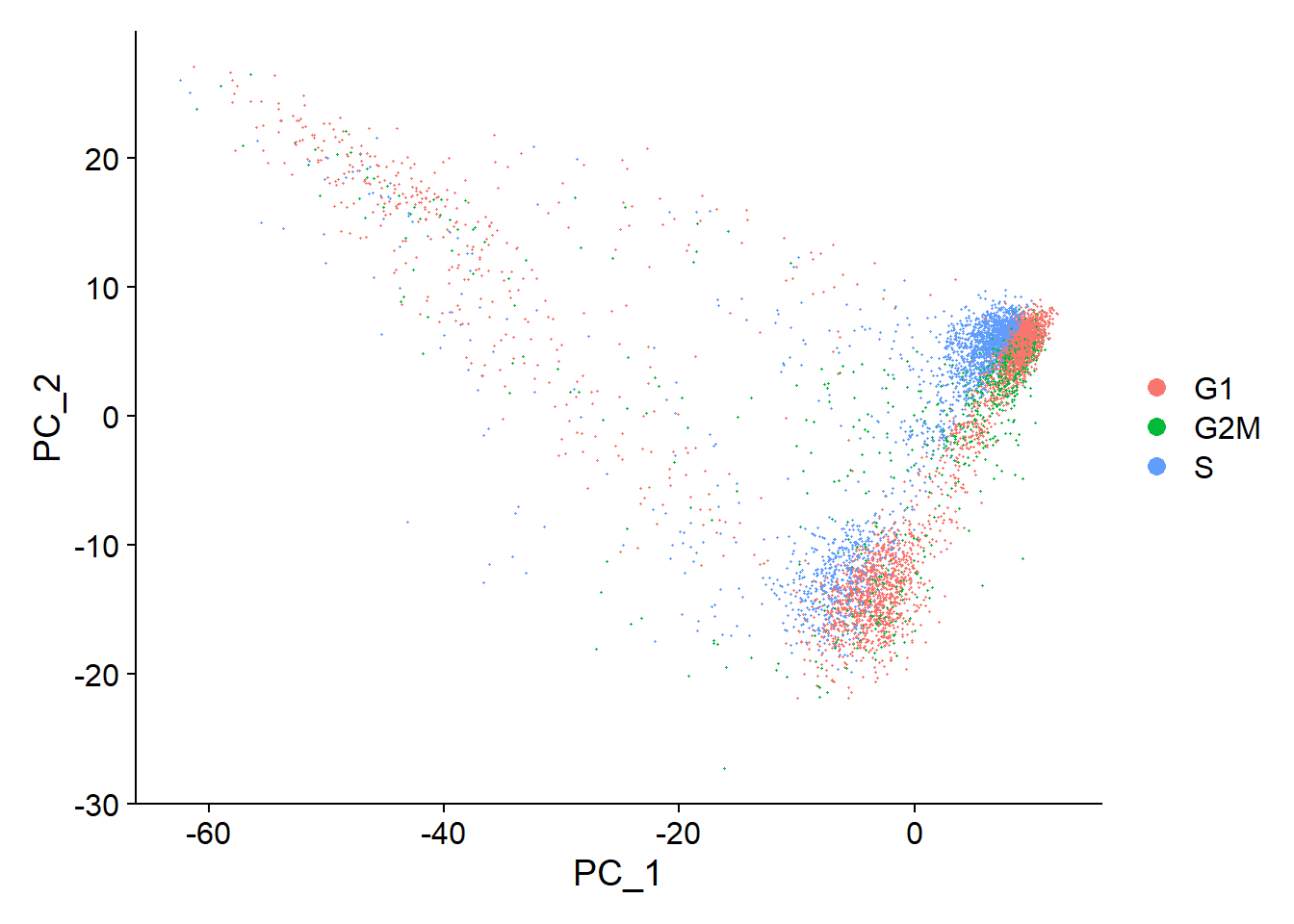
DimHeatmap(object = Fib, dims = 1:9, cells = 500, balanced = TRUE)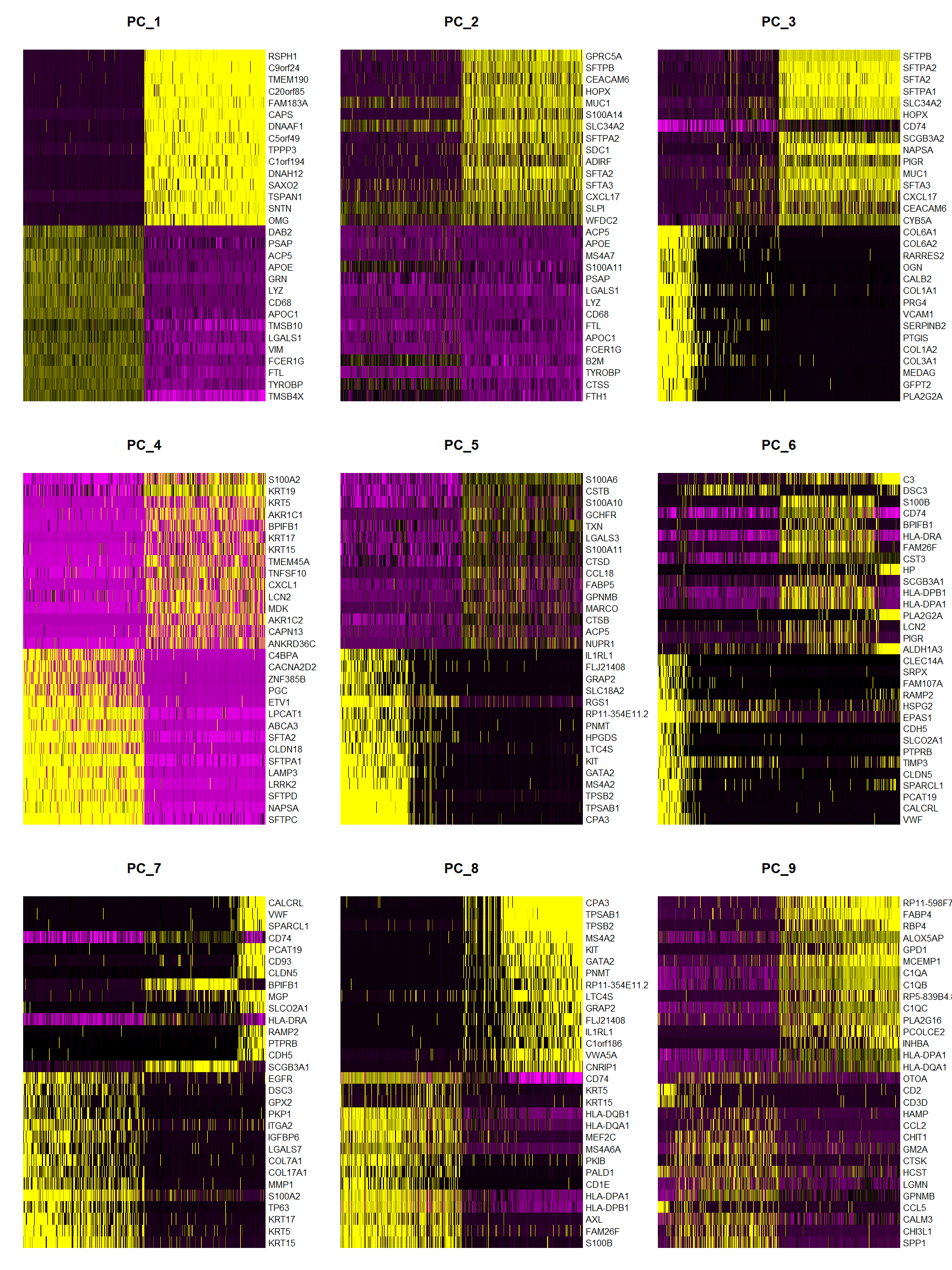
What is the ‘dimensionality’ of the data?
For clustering analyses we will choose the principal components which explain most of the variation in our data. Elbow plot uses a ranking of principle components based on the percentage explained by each one.
ElbowPlot(object = Fib)
We did not get a clear elbow shape here, but after 10th principal component additional dimensions do not explain big amount of the variance. So we will use first 10 dimensions for the subsequent analyses.
Cluster the cells
A graph-based clustering approach will be performed, built upon initial strategies in (Macosko et al).
Fib <- FindNeighbors(object = Fib, dims = 1:10)
Fib <- FindClusters(object = Fib, resolution = 0.5)
## Modularity Optimizer version 1.3.0 by Ludo Waltman and Nees Jan van Eck
##
## Number of nodes: 6320
## Number of edges: 196713
##
## Running Louvain algorithm...
## Maximum modularity in 10 random starts: 0.8872
## Number of communities: 15
## Elapsed time: 0 seconds# Look at cluster IDs of the first 5 cells
head(Idents(Fib), 5)## AAACCTGAGATCCCGC-1 AAACCTGAGCCAGAAC-1 AAACCTGAGGGATGGG-1
## 2 2 8
## AAACCTGAGTCGTACT-1 AAACCTGAGTCGTTTG-1
## 0 10
## Levels: 0 1 2 3 4 5 6 7 8 9 10 11 12 13 14TSNE plot
Fib <- RunTSNE(object = Fib, dims = 1:6)
DimPlot(object = Fib, reduction = 'tsne', label = TRUE, label.size = 5)
How to find genes that differentiate each cluster?
We can use FindMarkers() function to search for cluster biomarkers.
# Find all markers of cluster 0
cluster0.markers <- FindMarkers(object = Fib, ident.1 = 0, min.pct = 0.25)
head(x = cluster0.markers, n = 10)
## p_val avg_logFC pct.1 pct.2 p_val_adj
## GPNMB 0 1.0814399 0.947 0.450 0
## CSTB 0 1.0377160 0.994 0.892 0
## FTL 0 1.0160962 1.000 0.998 0
## APOC1 0 0.9919471 0.991 0.819 0
## SH3BGRL3 0 0.9252345 0.990 0.798 0
## CTSD 0 0.9105122 0.995 0.836 0
## FTH1 0 0.8873914 1.000 0.997 0
## PSAP 0 0.8835586 1.000 0.876 0
## CTSB 0 0.8773872 0.986 0.752 0
## LGALS1 0 0.8622147 0.992 0.637 0# Find markers for every cluster compared to all remaining cells, report only
# the positive ones
Fib.markers <- FindAllMarkers(object = Fib, only.pos = TRUE, min.pct = 0.25,
logfc.threshold = 0.25)
# Make a table containing markers for each cluster set.
# We will use this table to assign cell types to clusters.
Fib.markers %>% group_by(cluster) %>% top_n(n = 5, wt = avg_logFC) %>%
print(n = 85)## # A tibble: 75 x 7
## # Groups: cluster [15]
## p_val avg_logFC pct.1 pct.2 p_val_adj cluster gene
## <dbl> <dbl> <dbl> <dbl> <dbl> <fct> <chr>
## 1 0. 1.08 0.947 0.45 0. 0 GPNMB
## 2 2.60e-293 1.13 0.935 0.582 5.27e-289 0 FABP5
## 3 8.54e-289 1.12 0.814 0.365 1.73e-284 0 CTSL
## 4 3.43e-188 1.43 0.46 0.133 6.95e-184 0 SPP1
## 5 2.78e-110 1.37 0.288 0.078 5.64e-106 0 CCL2
## 6 2.69e-231 1.33 0.996 0.658 5.45e-227 1 APOE
## 7 1.91e-204 1.02 0.926 0.403 3.86e-200 1 MS4A6A
## 8 1.35e-174 0.918 0.932 0.423 2.74e-170 1 C1QC
## 9 1.59e-119 1.07 0.86 0.457 3.22e-115 1 CCL18
## 10 1.56e- 56 0.916 0.576 0.311 3.15e- 52 1 SEPP1
## 11 0. 2.26 0.663 0.108 0. 2 FABP4
## 12 0. 1.43 0.846 0.165 0. 2 MCEMP1
## 13 5.19e-222 1.24 0.969 0.496 1.05e-217 2 GCHFR
## 14 4.41e-218 1.36 0.98 0.505 8.93e-214 2 C1QA
## 15 4.43e-210 1.35 0.967 0.483 8.97e-206 2 C1QB
## 16 0. 3.18 0.964 0.339 0. 3 SCGB3A2
## 17 0. 2.01 0.995 0.376 0. 3 SFTPB
## 18 0. 1.73 0.943 0.188 0. 3 CEACAM6
## 19 2.27e-273 2.23 0.929 0.364 4.59e-269 3 SFTPA2
## 20 8.38e-271 1.72 0.813 0.203 1.70e-266 3 SFTPA1
## 21 0. 2.70 0.896 0.035 0. 4 C9orf24
## 22 0. 2.46 0.87 0.026 0. 4 TMEM190
## 23 0. 2.44 0.892 0.026 0. 4 RSPH1
## 24 0. 2.42 0.868 0.025 0. 4 C20orf85
## 25 0. 2.39 0.907 0.104 0. 4 TPPP3
## 26 0. 2.76 0.975 0.227 0. 5 S100A2
## 27 0. 2.19 0.797 0.083 0. 5 KRT15
## 28 0. 1.72 0.684 0.048 0. 5 KRT5
## 29 6.72e-278 1.93 0.471 0.035 1.36e-273 5 MMP1
## 30 9.96e-220 1.75 0.925 0.319 2.02e-215 5 AQP3
## 31 0. 2.45 0.737 0.077 0. 6 BPIFB1
## 32 6.07e-262 2.14 0.984 0.305 1.23e-257 6 WFDC2
## 33 2.03e-221 2.21 0.982 0.385 4.11e-217 6 SLPI
## 34 1.17e-163 3.21 0.948 0.624 2.36e-159 6 SCGB3A1
## 35 8.07e-152 2.91 0.797 0.293 1.63e-147 6 SCGB1A1
## 36 0. 2.57 0.797 0.072 0. 7 S100B
## 37 9.62e-289 1.76 0.829 0.156 1.95e-284 7 FAM26F
## 38 2.50e-224 2.18 1 0.728 5.06e-220 7 HLA-DPB1
## 39 2.51e-213 1.99 0.992 0.658 5.07e-209 7 HLA-DPA1
## 40 1.75e-191 1.71 0.955 0.449 3.55e-187 7 HLA-DQA1
## 41 4.11e- 50 1.01 0.546 0.231 8.31e- 46 8 STMN1
## 42 1.29e- 41 0.917 0.819 0.529 2.60e- 37 8 TUBA1B
## 43 1.29e- 40 0.915 0.807 0.517 2.61e- 36 8 TUBB
## 44 1.32e- 29 0.973 0.825 0.615 2.67e- 25 8 H2AFZ
## 45 5.14e- 29 1.16 0.77 0.503 1.04e- 24 8 HIST1H4C
## 46 0. 2.28 0.984 0.113 0. 9 NAPSA
## 47 3.65e-299 2.20 0.984 0.159 7.39e-295 9 SFTA2
## 48 8.60e-252 2.99 1 0.226 1.74e-247 9 SFTPA1
## 49 3.66e-220 4.21 0.961 0.265 7.42e-216 9 SFTPC
## 50 4.19e-168 2.33 0.992 0.39 8.47e-164 9 SFTPA2
## 51 0. 2.61 0.570 0.01 0. 10 COL3A1
## 52 0. 2.56 0.604 0.005 0. 10 SPARCL1
## 53 0. 2.42 0.456 0.005 0. 10 PLA2G2A
## 54 0. 2.40 0.544 0.005 0. 10 COL1A2
## 55 1.09e-278 2.57 0.537 0.02 2.20e-274 10 COL1A1
## 56 0. 4.23 0.993 0.035 0. 11 TPSB2
## 57 0. 3.74 0.993 0.02 0. 11 TPSAB1
## 58 0. 3.32 1 0.02 0. 11 CPA3
## 59 0. 2.78 0.911 0.017 0. 11 MS4A2
## 60 0. 2.33 0.856 0.016 0. 11 KIT
## 61 1.98e-262 2.08 0.624 0.023 4.01e-258 12 FCN1
## 62 5.17e- 70 1.95 0.475 0.059 1.05e- 65 12 IL1R2
## 63 2.47e- 66 1.98 0.634 0.119 5.01e- 62 12 VCAN
## 64 4.37e- 58 3.03 0.812 0.258 8.85e- 54 12 S100A8
## 65 2.45e- 46 2.67 0.901 0.466 4.96e- 42 12 S100A9
## 66 2.37e- 68 2.24 0.593 0.055 4.80e- 64 13 IL32
## 67 1.03e- 66 2.00 0.296 0.013 2.08e- 62 13 KLRB1
## 68 4.82e- 52 3.79 0.259 0.013 9.77e- 48 13 IGHG1
## 69 3.98e- 44 3.37 0.259 0.015 8.06e- 40 13 IGHG4
## 70 3.42e- 42 2.22 0.352 0.03 6.92e- 38 13 CCL5
## 71 6.32e-208 1.85 0.978 0.036 1.28e-203 14 CPA3
## 72 1.19e-176 1.28 0.822 0.03 2.41e-172 14 KIT
## 73 3.11e-176 1.40 0.844 0.032 6.30e-172 14 MS4A2
## 74 7.63e-172 1.75 0.889 0.036 1.54e-167 14 TPSAB1
## 75 2.72e-158 2.05 0.978 0.051 5.50e-154 14 TPSB2For more details consult to DE vignette.
According to the table above I generated a cluster id vector to assign cell type to each cluster. I have a group NA which I could not assign a cell type, which is probably a technical artifact from cell cycle regression since the top genes expressed in this population are cell cycle related. I also found 3 subpopulations of macrophages and 2 types of mast cells in thiS patient.
# Assigning Cell ids

new.cluster.ids <- c("Macrophages(1)", "Macrophages(2)", "Macrophages(3)",
                     "AT2(1) Cells", "Cliated Cells", "Basal Cells", "Club Cells",
                     "Dendritic Cells", "NA", "AT2(2) Cells", "Fibroblasts",
                     "Mast(1) Cells", "Monocytes", "T/NKT Cells", "Mast(2) Cells")
names(new.cluster.ids) <- levels(Fib)
Fib <- RenameIdents(Fib, new.cluster.ids)
DimPlot(Fib, reduction = "tsne", label = TRUE, label.size = 8, pt.size = 1.0) + NoLegend()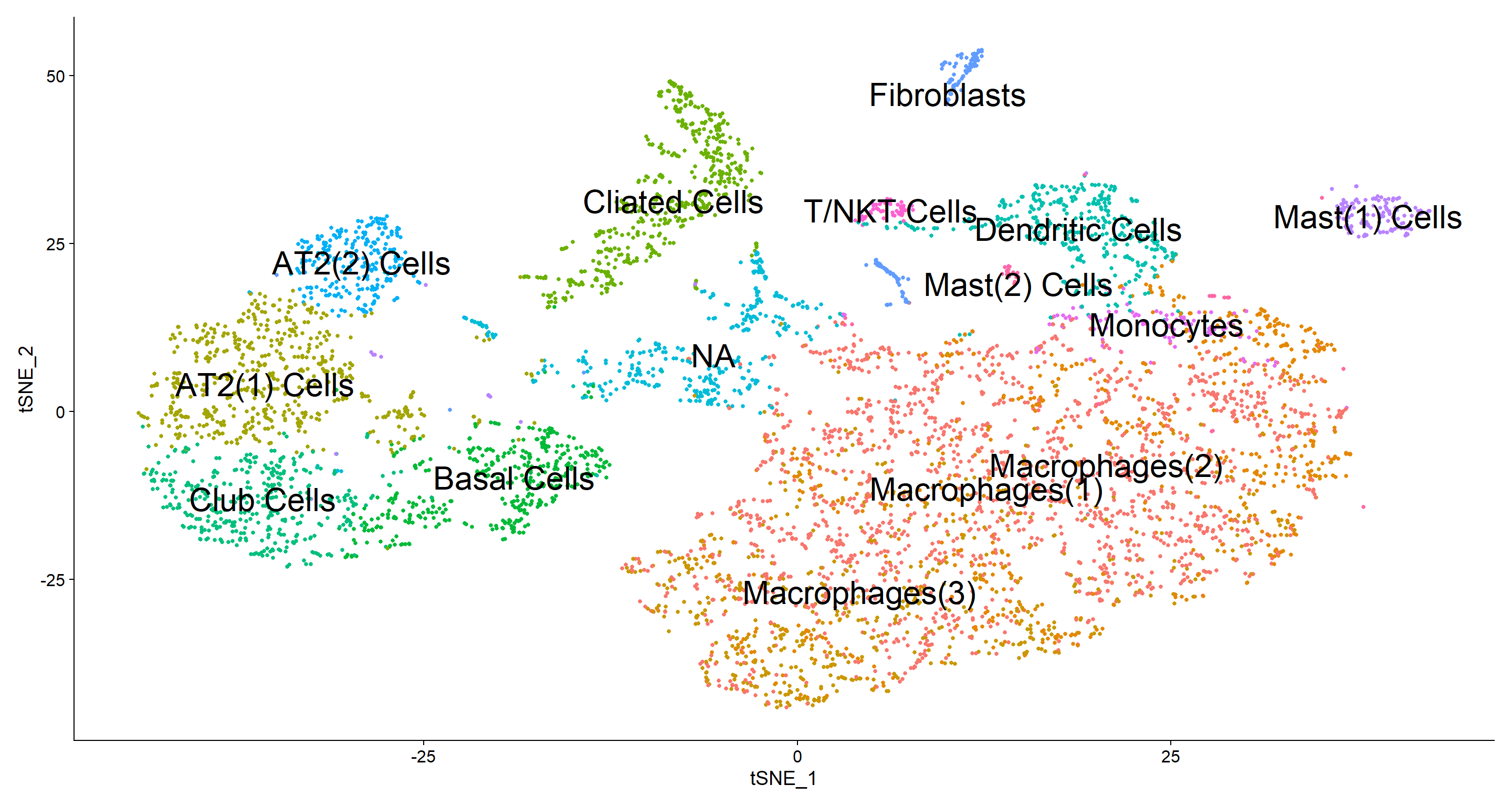
# Let's look at the expression of a few genes of interest accross different subtypes
VlnPlot(Fib, features = c("SPP1", "CHIT1"))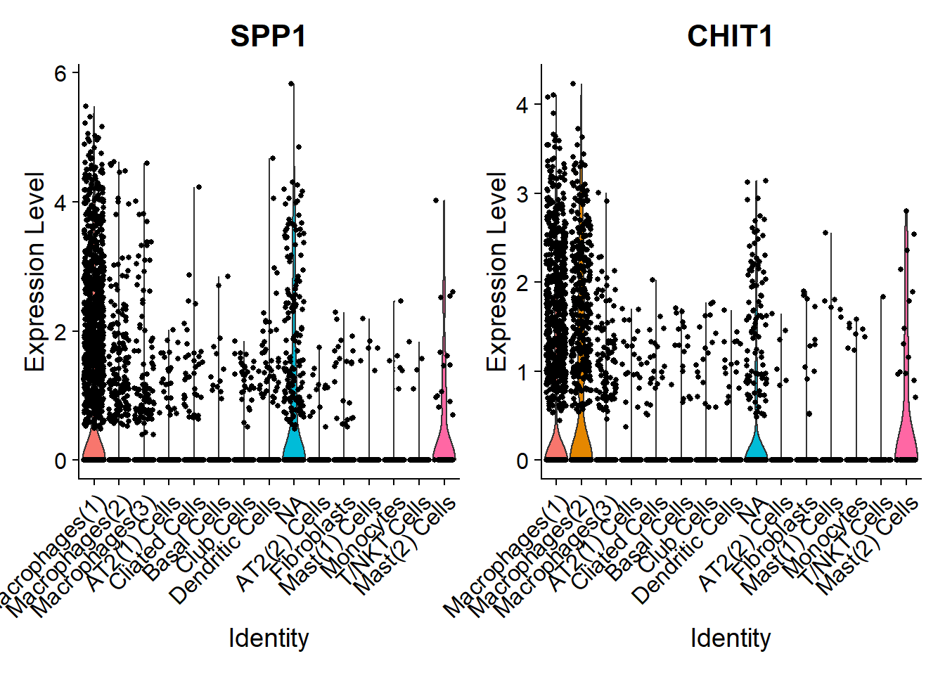
FeaturePlot(Fib, features = c("SPP1", "APOE", "SCGB3A2", "C9orf24", "S100A2", "BPIFB1", "S100B", "COL3A1", "FCN1"))
What cells Biotech Companies are targeting in lung fibrosis?
Novel therapies in pulmonary fibrosis are urgently needed. Let’s look at few promising drugs currently in clinical trials.
Fibrinogen
Fibrinogen’s lead compound pamrevlumab blocks CTGF. Let’s have a look which cells produce it.
VlnPlot(Fib, features =c("CTGF"))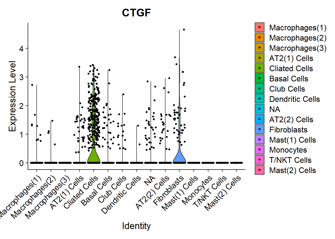
FeaturePlot(Fib, features = c("CTGF"), pt.size = 1)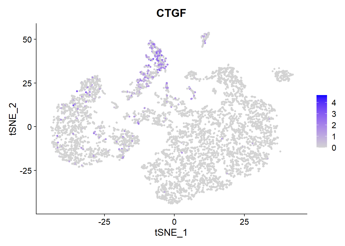 Main source for the
 CTGF production here seems the Ciliated cells.
Galapagos
Galapagos GLPG1690 has entered Phase 3 clinical trials and it targets Autotaxin (ENPP2).
VlnPlot(Fib, features = c("ENPP2"))
FeaturePlot(Fib, features = c("ENPP2"), pt.size = 1)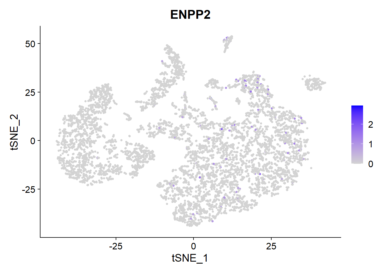 We see a low expression of
 ENPP mainly in Macrophages, Dendritic cells and Fibroblasts.
The other clinical candidate of Galapagos is GLPG1205 which targets GPR84. It has entered Phase 2 clinical trials.
VlnPlot(Fib, features = c("GPR84"))
FeaturePlot(Fib, features = c("GPR84"), pt.size = 1)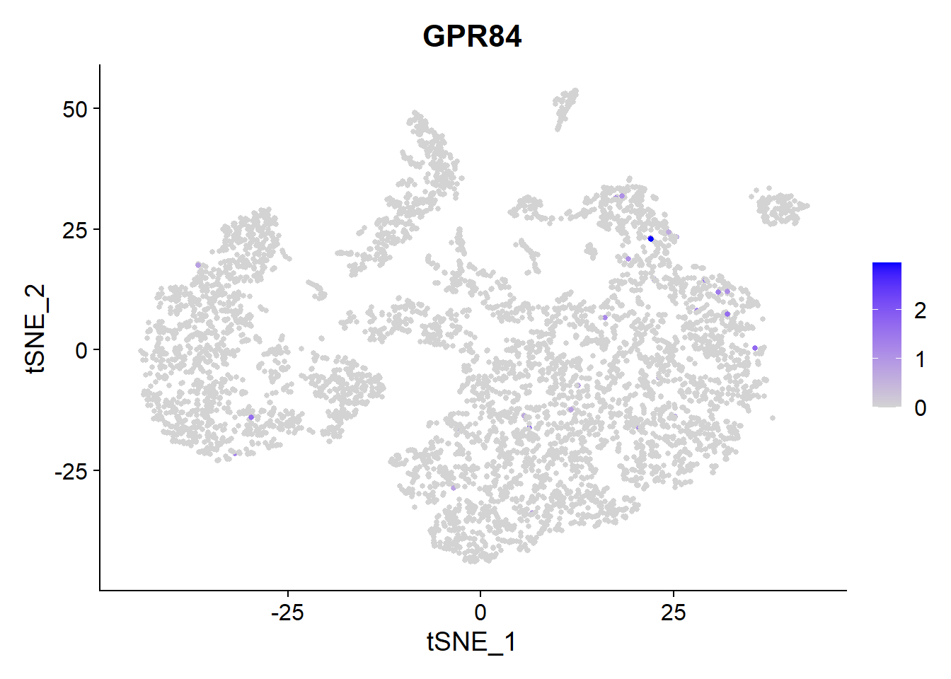
GPR84 has very low expression throughout the lung cells of this patient. The gene is mainly expressed in Type 1 Macrophages.
Bristol-Myers-Squibb: BMS-986020
BMS-986020 is an anti-fibrotic drug being developed by Bristol-Myers Squibb, and is a lysophosphatidic acid (LPA) receptor antagonist.
Let’s look at the expression of a LPAR1.
VlnPlot(Fib, features = c("LPAR1"))
FeaturePlot(Fib, features =c("LPAR1"), pt.size = 1)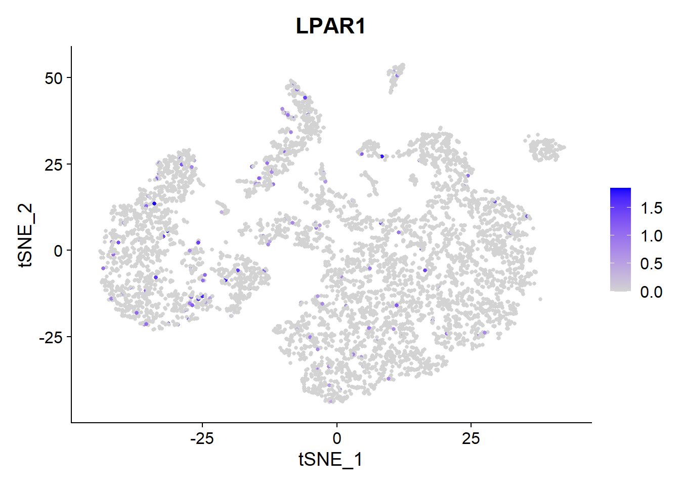 It is expressed at low levels but consistently on many types of lung cells.
Roche nintedanib
Nintedanib is one of the two new medicines approved for IPF patients. It targets multiple receptor tyrosine kinase receptors such as VEGF, FGF and PDGF.
VlnPlot(Fib, features = c("VEGFA", "PDGFA"))
FeaturePlot(Fib, features = c("VEGFA", "PDGFA"), pt.size = 1)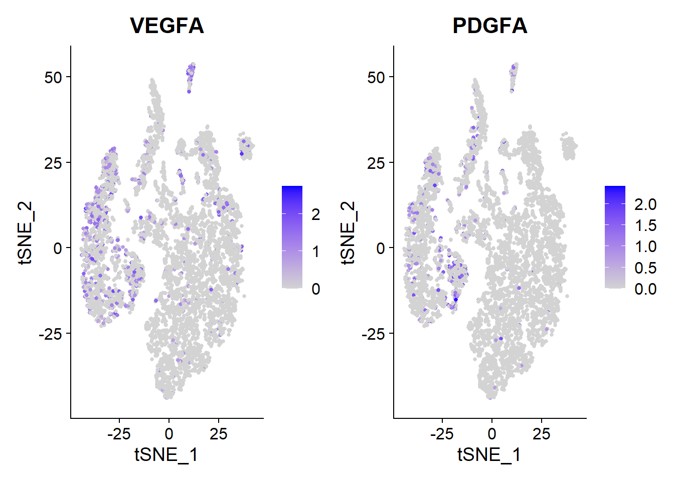
VEGFA, PDGFA is highly expressed in multiple types of cells in the lung microenvironment.
Final thoughts
Seurat package allowed us to cluster different types of lung cells so that we can visualize their specific gene expression. We used those plots to see which cells express the drug targets in clinical trials or in use.
Although changes associated with fibrosis are well defined the causal factors are not known. Reflecting this we saw that those drugs target many different components of the lung microenvironment. The conquest is on and we hope promising therapies arrive soon.